MAE 4190 | Fast Robots
Jueun Kwon
Jueun Kwon
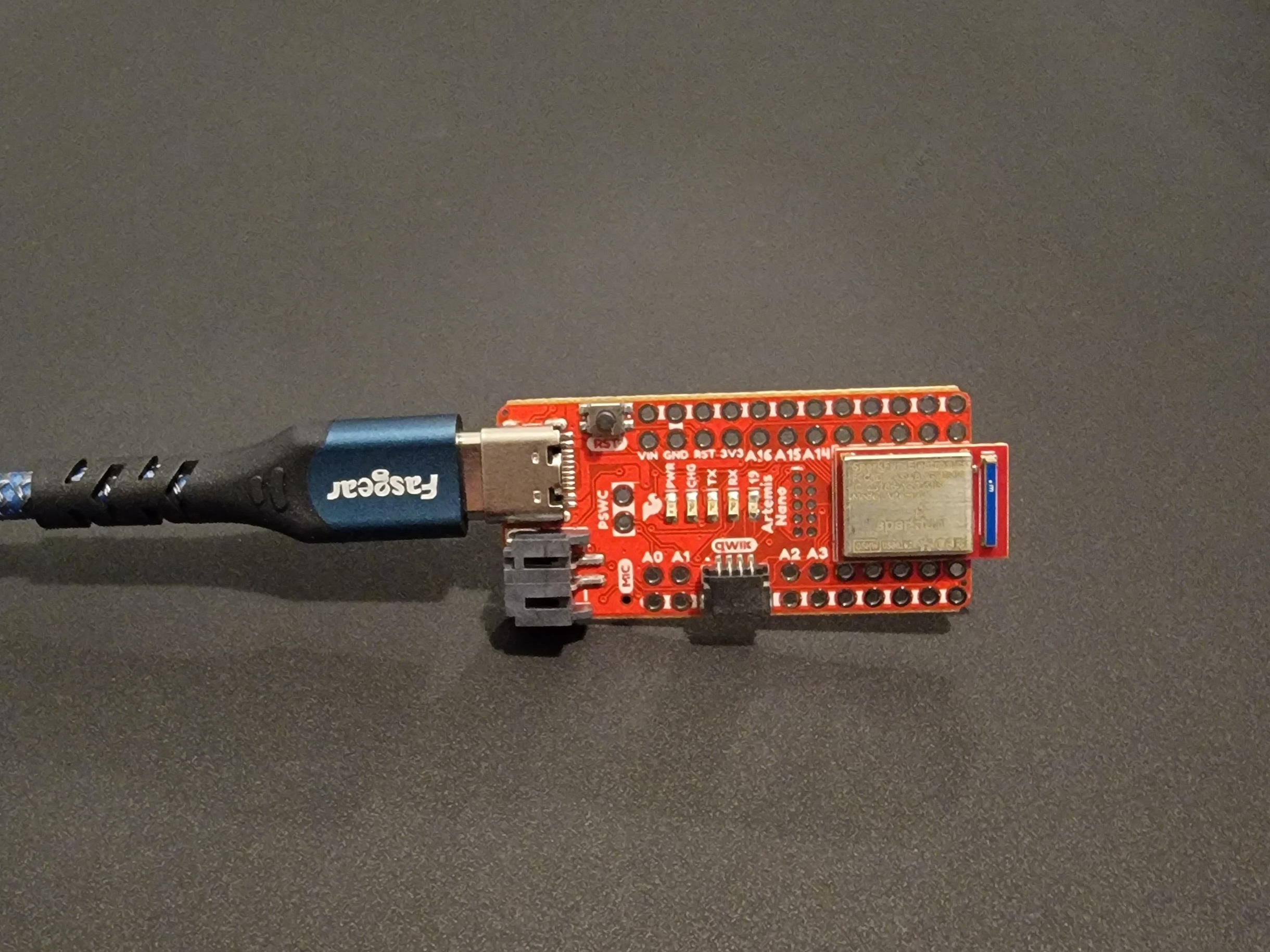

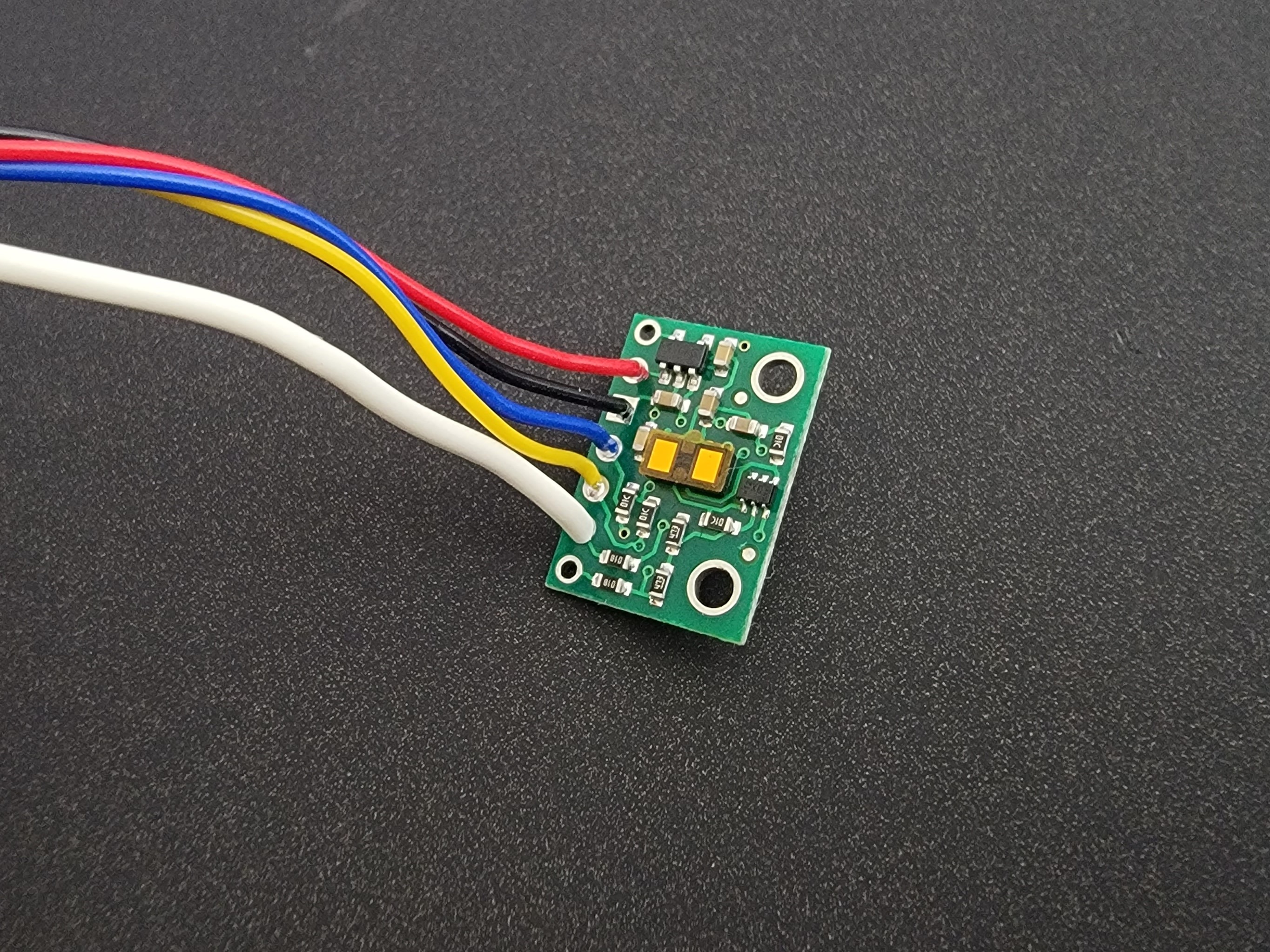
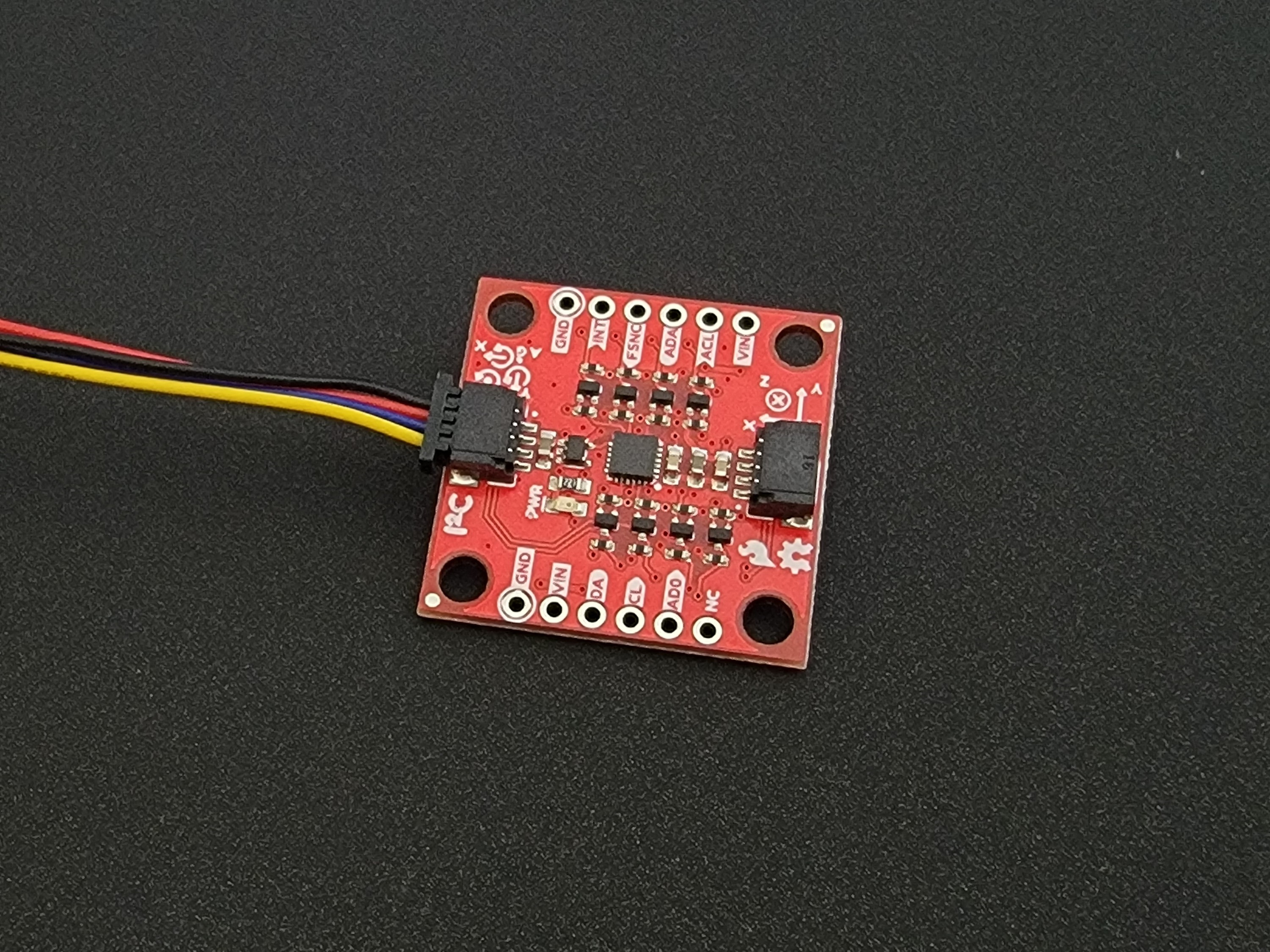
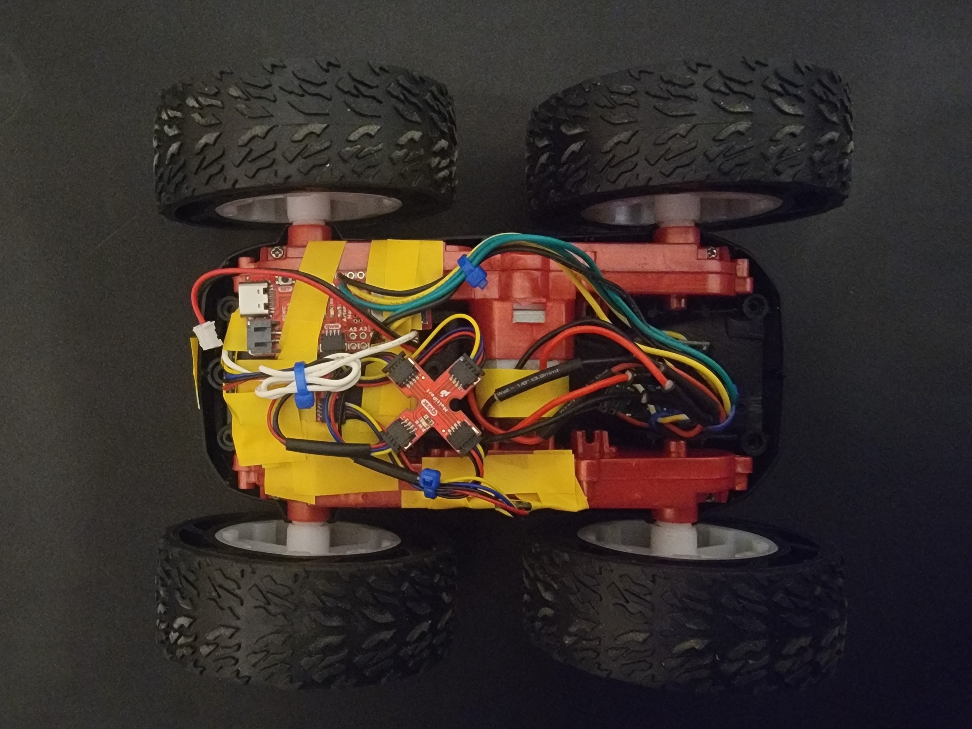

Hello! My name is Jueun Kwon, and I am a junior mechanical engineering student at Cornell University. I am passionate about applying mechanical engineering and robotics concepts to various fields such as autonomous systems, hardware, and product design.

The goal of this lab was to get setup with Arduino and Appollo3 software, as well as to get comfortable using the Artemis board.
I hooked up the Artemis board to my computer and followed the step by step instruction from this link. I uploaded the code found from "File->Examples->01.Basics->Blink" to the board and lowered the baud rate to 115200 bits per second in order to make the board blink.
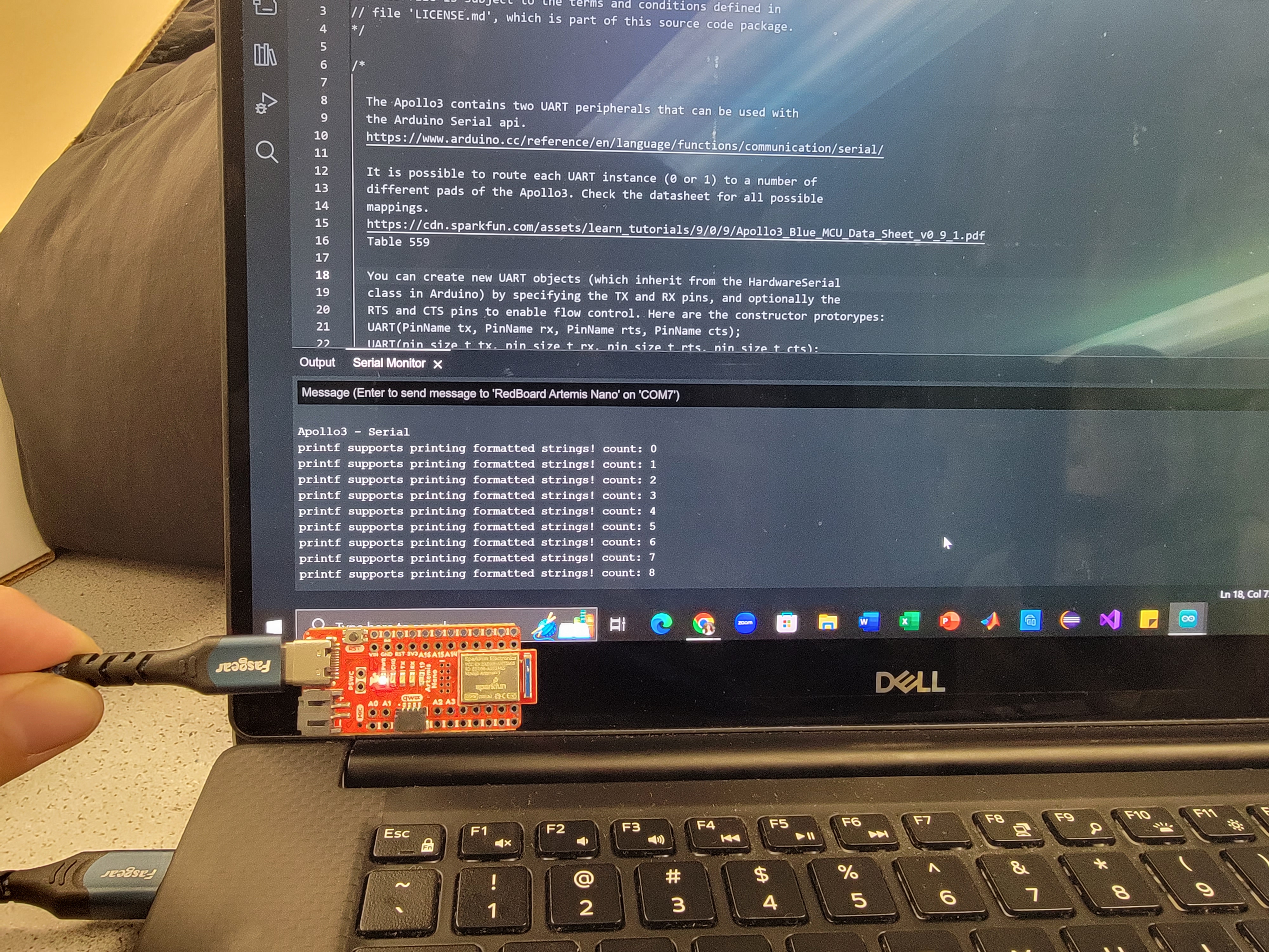
I uploaded the code found from "File->Examples->Apollo3->Example01_Serial" to the board. The serial communication between Artemis and the computer was tested and shown on the serial monitor. I was able to provide input and view the output as well.
I uploaded the code found from "File->Examples->Apollo3->Example02_AnalogRead" to test the sensors on the board. The serial monitor printed the sensor readings for analog voltage, temp, Vcc, Vss, and time. For the purpose of this lab, I focused on the temperature sensor. The temperature readings went up when I put my finger on the chip and down when I removed my finger from the chip.
I uploaded the code found from "File->Examples->PDM->Example1_MicrophoneOutput" to test my microphone. I observed in the serial monitor that the frequency went up when I whistled at the board.
The goal of this lab is to establish bluetooth communication and transfer data between the computer and the arthemis board.
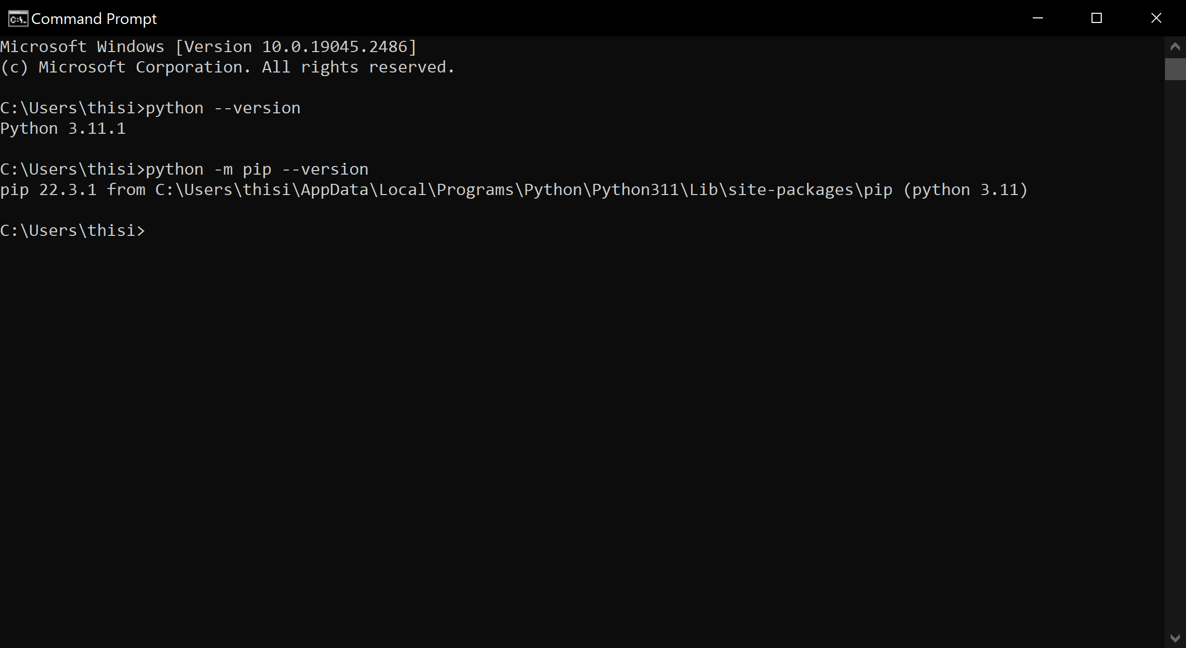
I learned about the basics of a BLE through this link. I installed python3, pip, jupyter, and set up the "FastRobots_ble" virtual environment. Then, I checked to make sure I downloaded a Python >= 3.9 and pip >= 21.
I installed and burned the sketch ble_arduino.ino from the codebase. From this, I was able to identity my MAC address.
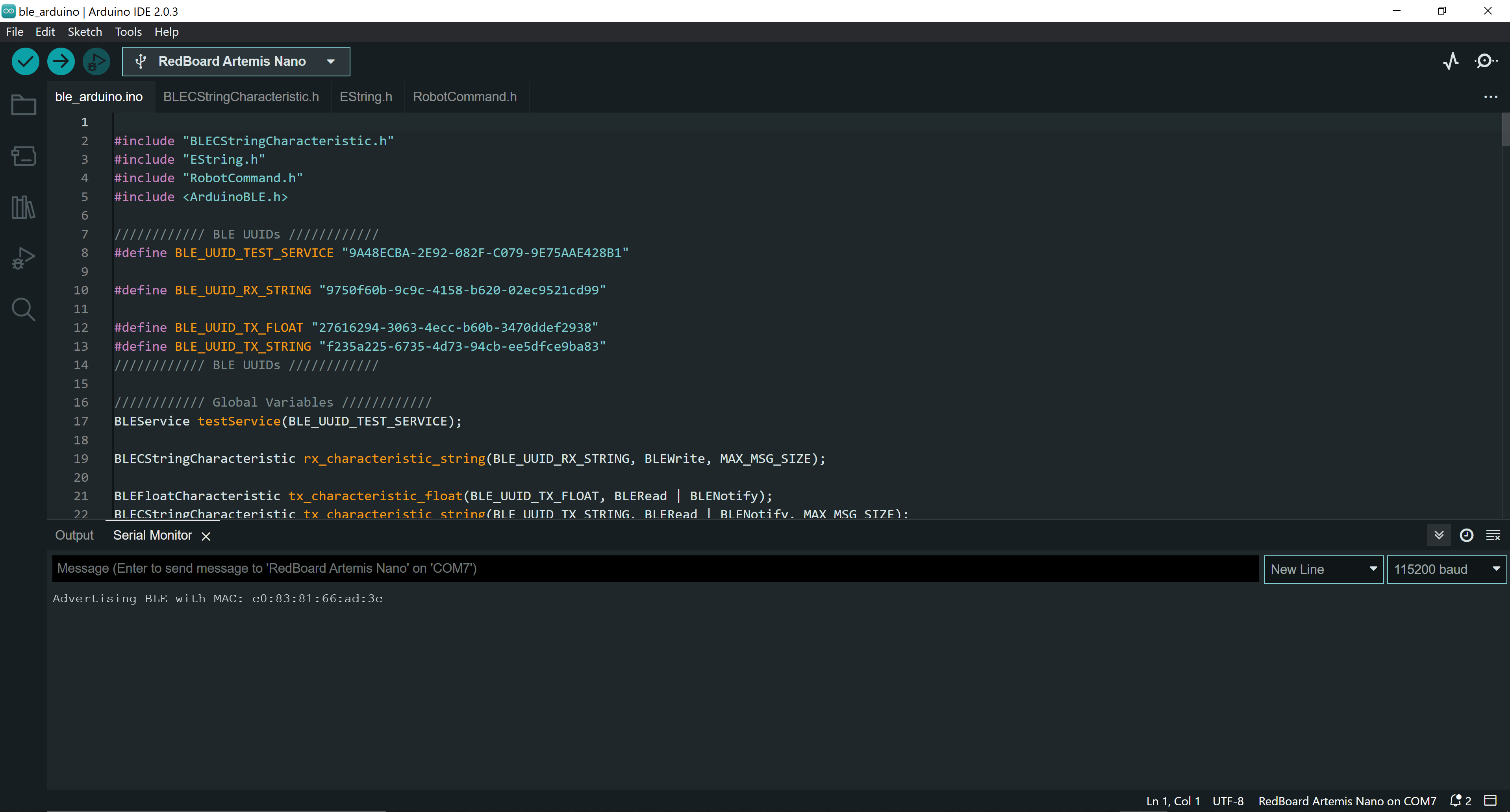
The codebase includes all the necessary files to let my computer communicate with the artemis board via bluetooth. The codebase can be viewed mainly in two parts: ble_arduino and ble_python. ble_arduino includes set up code and arduino code that will run on the artemis board. ble_python includes all set up code and jupyter notebook to run all the commands.
ArdunioBLE uses Bluetooth LE radio that works like a bulletin board, shared between the computer and the arthemis board. If the arthemis posts data on the bulletin board, my computer can read the data posted on the bulletin board.
Starting Bluetooth:
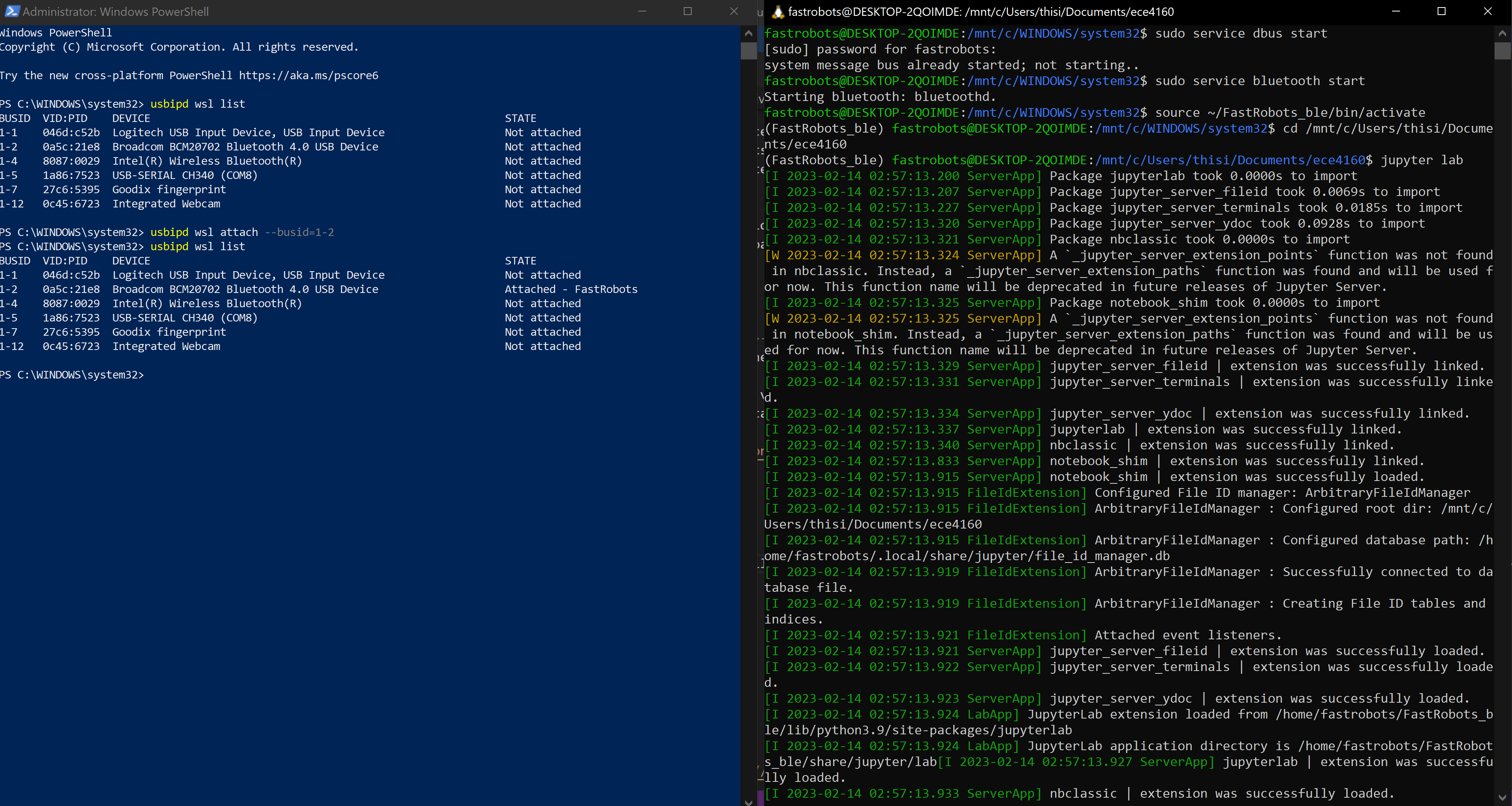
Because I couldn't get my artemis to connect via my original bluetooth module on my laptop, I used the plugable usb and enabled the additional bluetooth module via WSL.
I run the following commands everytime I restart bluetooth and open my jupyter lab:
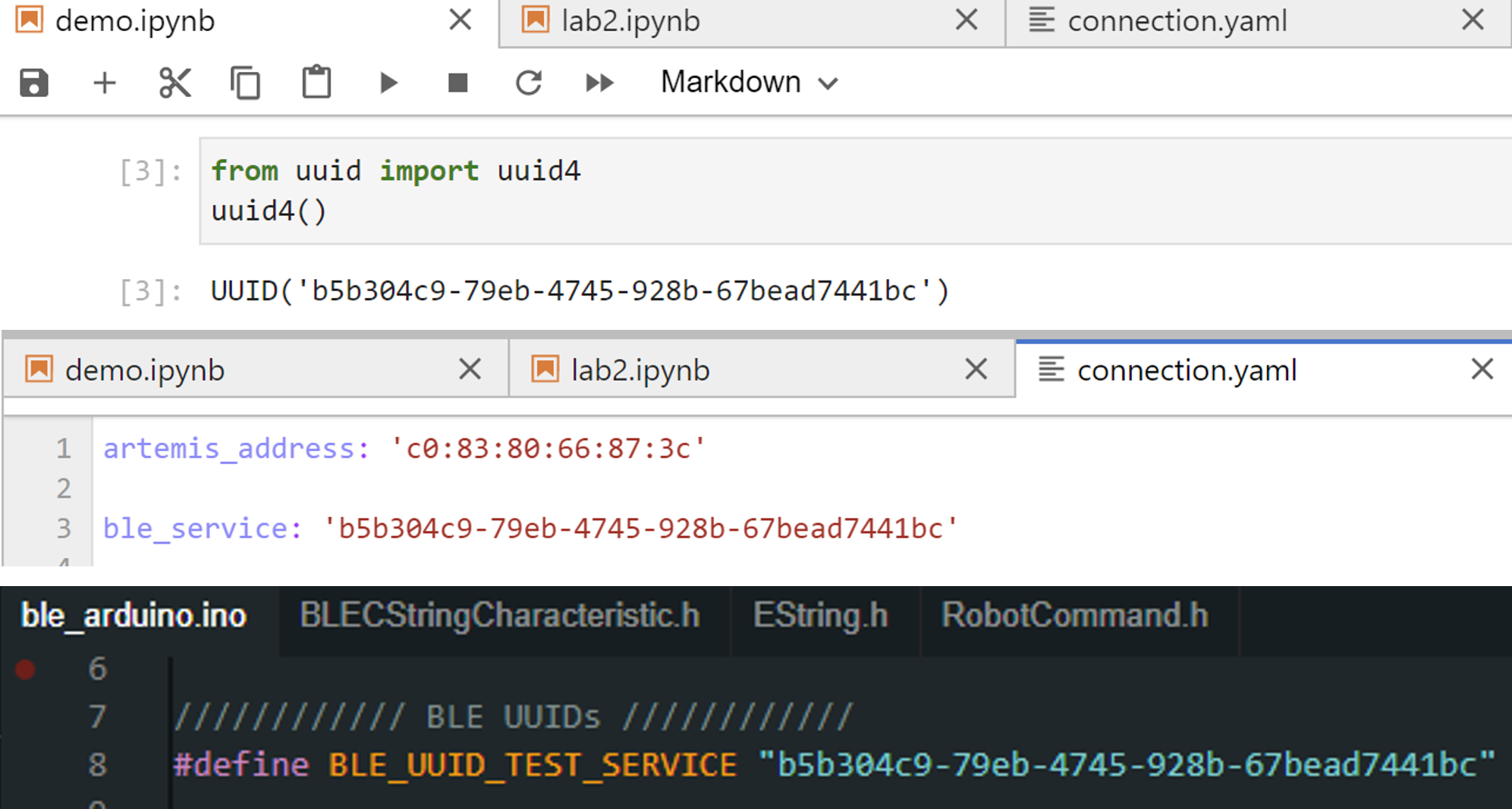
In connections.yaml, I replaced the artemis_address value to match the MAC address given by my Artemis (shown in the pre section). In addition, I generated a new BLEService UUID from the juypter lab and updated connections.yaml and ble_aruino.ino to match this address.
demo.ipynb:
I checked that everything in the demo.ipynb file is working as intended. A runthrough of my demo is shown below:
Echo command sends a string from the computer to the artemis board. Then, the computer receives a string from the artemis board.
>
GET_TIME_MILLIS command was added to get the time from the artemis board.

A notification handler was created to recieve string data from the artemis board and return the time.

GET_TEMP_5s command was added to get five timestamped internal die temperature reading from the artemis board. The temperature reading was taken once every second for five seconds.

GET_TEMP_5s command was added to get as many temperature data as possible in 5 seconds. A notification handler was used to manage data.
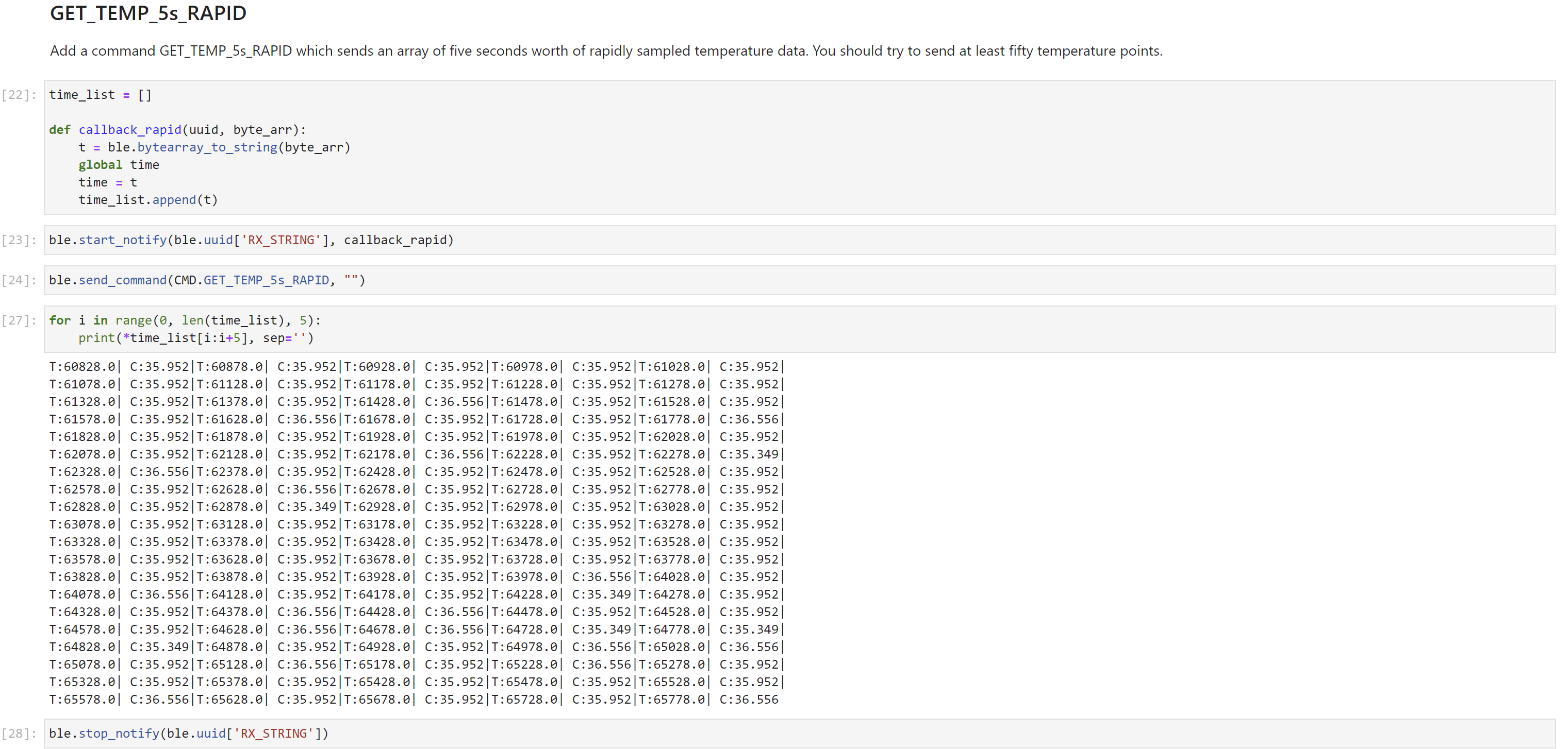
Working with strings introduces a huge latency, so it is better to transer data in chunks.
The artemis board has 385 kB of RAM. There are 8 bits in a byte and 1000 bytes in 1 kB.
So, artemis board has 385 x 1000 x 8 = 3080000 bits of RAM.
If we were to take 16 bit values at 150 Hz, that means we are taking 150 samples per second of the 16 bit data.
(150 samples/seconds) x (16 bit) = 2400 bit per second.
That means, we can theortically send 3080000/2400 = 1283.3 seconds of 16 bit values taken at 150Hz.
Since this is the theortical value, our limit would be less than 1283.3 seconds of 16 bit values taken at 150Hz.
The goal of this lab is to be able to use two ToF sensors at the same time and transfer ToF sensor data to the computer over bluetooth.
The default I2C sensor address, noted in the ToF sensor manual, is 0x52.

In order to use 2 ToF sensor, the sensor's address can be changed (while powered on) or the two sensors can be enabled alternatingly, with the use of their corresponding shutdown pins. I will take the former approach due to efficeny of changing the address once at the start of every run.
Given the sensor's range and angular sensitivity, I am planning to mount one ToF sensor to the front of the car and one to the side of the car. This means, I won't be detect obstacles on one of the sides and on the back.
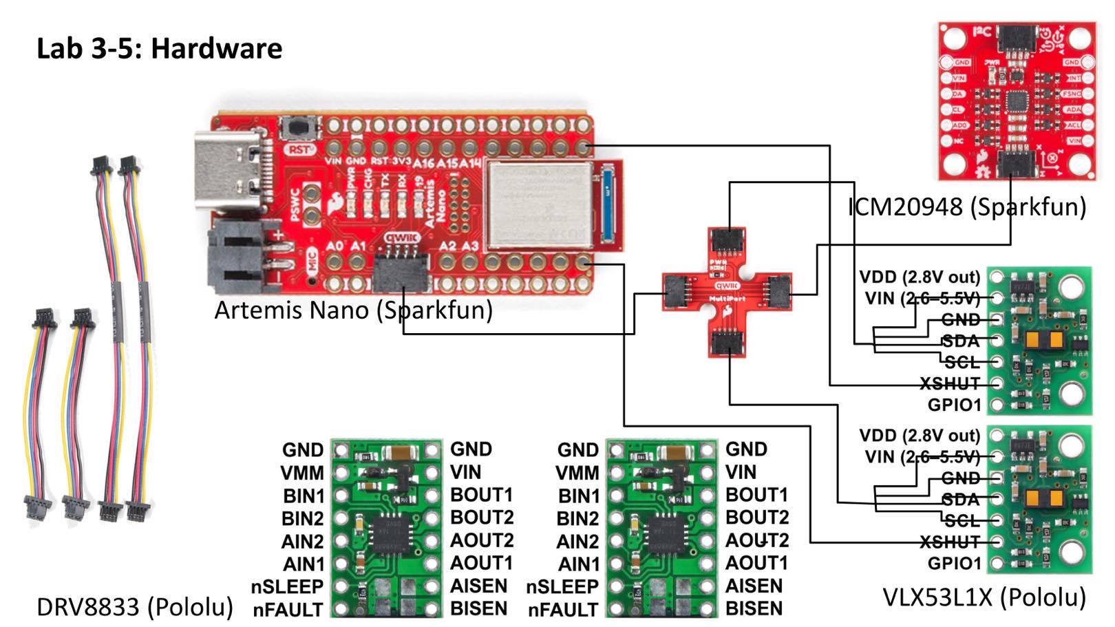
Below is a sketch of my wiring diagram.
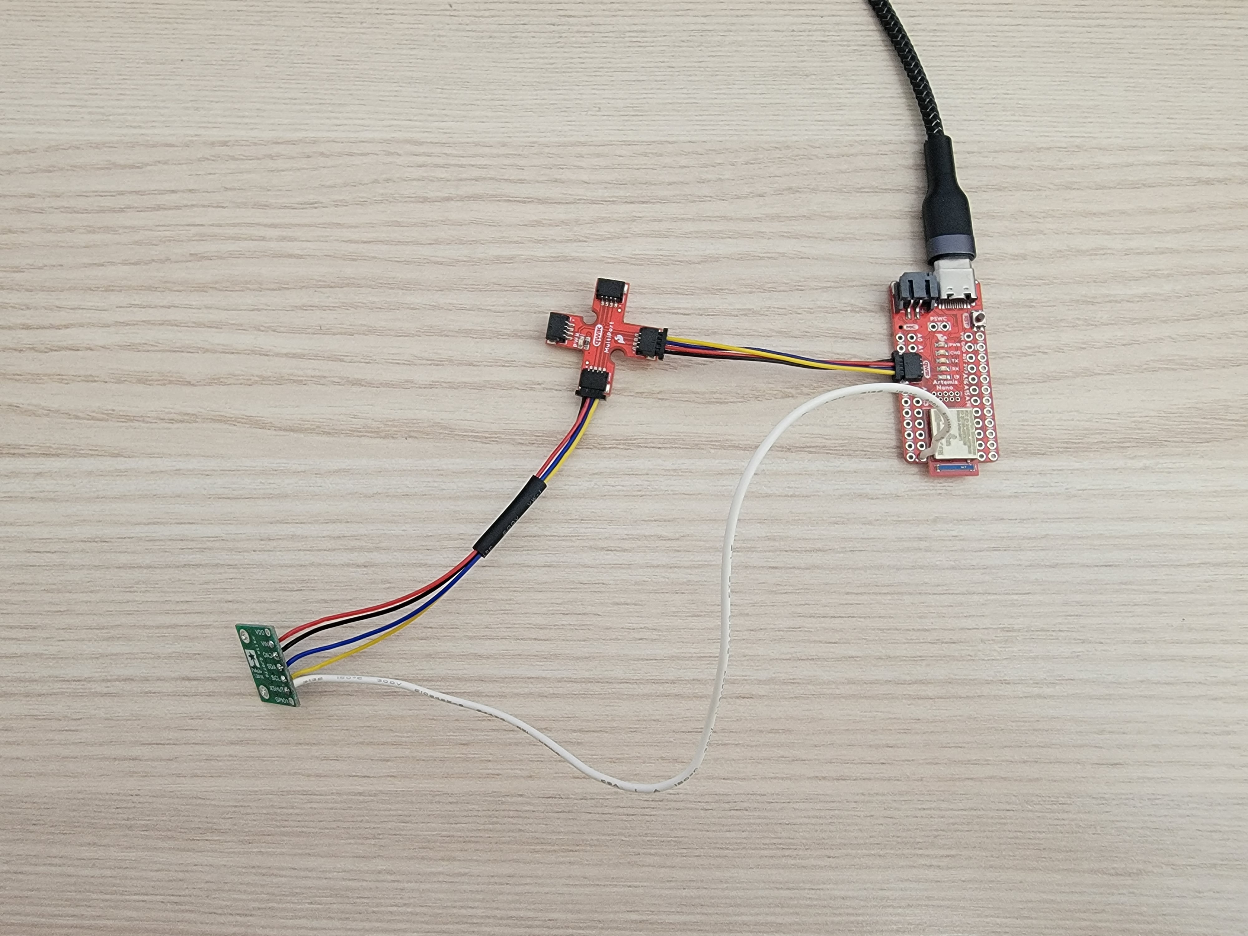
Below is my ToF sensor connected to your QWIIC breakout board and the Arthemis board.
I uploaded the code found from "File -> Examples -> Apollo3- > Example05_Wire_I2C" to the board to scan for the I2C address. The I2C address was read as 0x29 (or 0b11101) in the serial monitor.
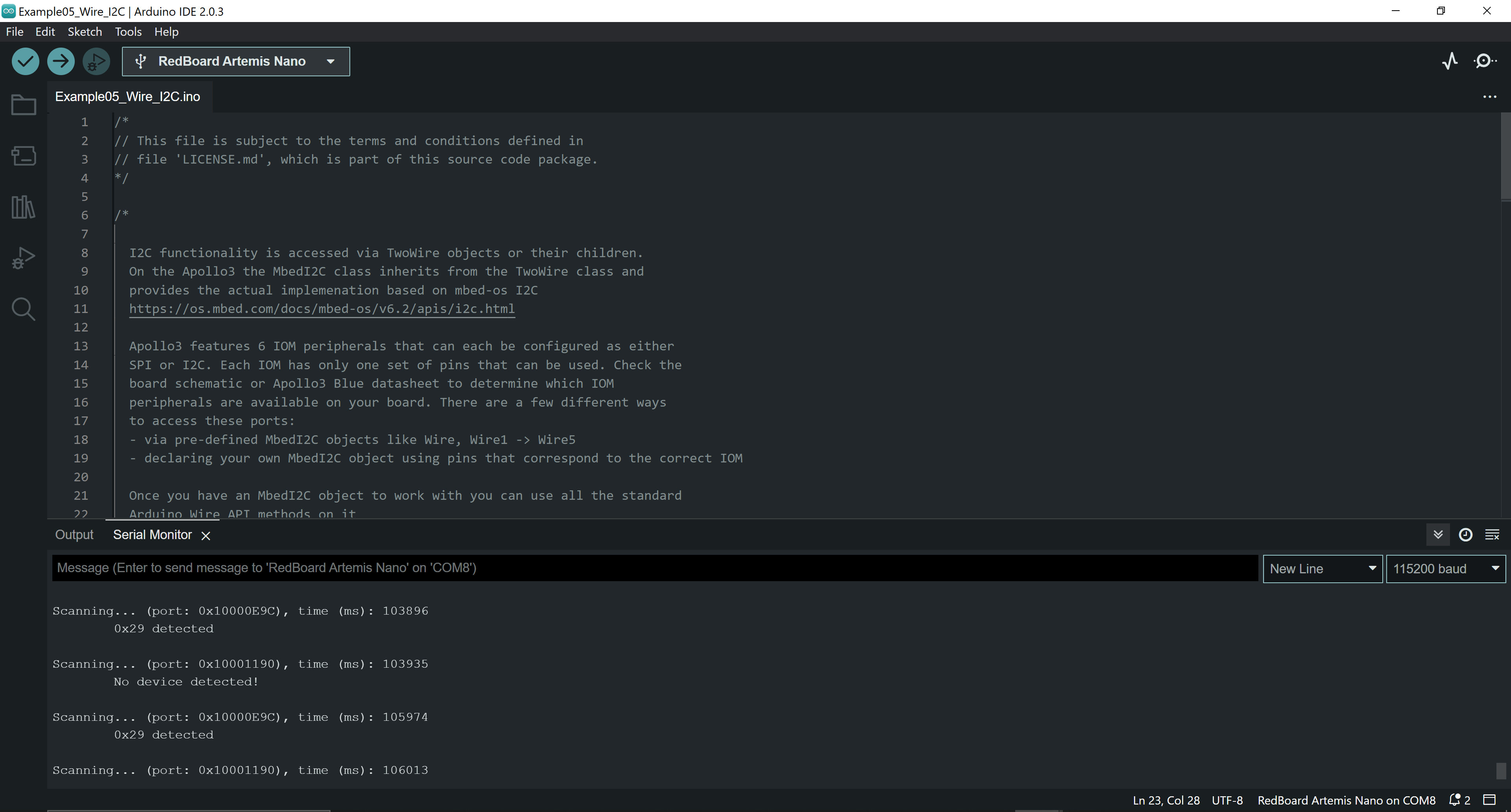
However, we have to shift this by 1 bit because the sensor contains an LSBit at the end of the 7 bit address. So, 0b11101 becomes 0b110100, which is 0x52.

The ToF sensor has three distance modes: short, medium, and long. Short distance mode has a a maximum distance of 136cm in dark and 135 in ambient light. Long distance mode has a maximum distance of 360cm in dark and 73 in ambient light. I chose to use the short distance mode since it is more immune to various lighting conditions.

I uploaded the code found from "File -> Examples -> SparkFun VL53L1X 4m Laser Distance Senseor -> Example1_ReadDistance" to the board to test my chosen distance mode. Below is my set up to test my sensor's accuracy.
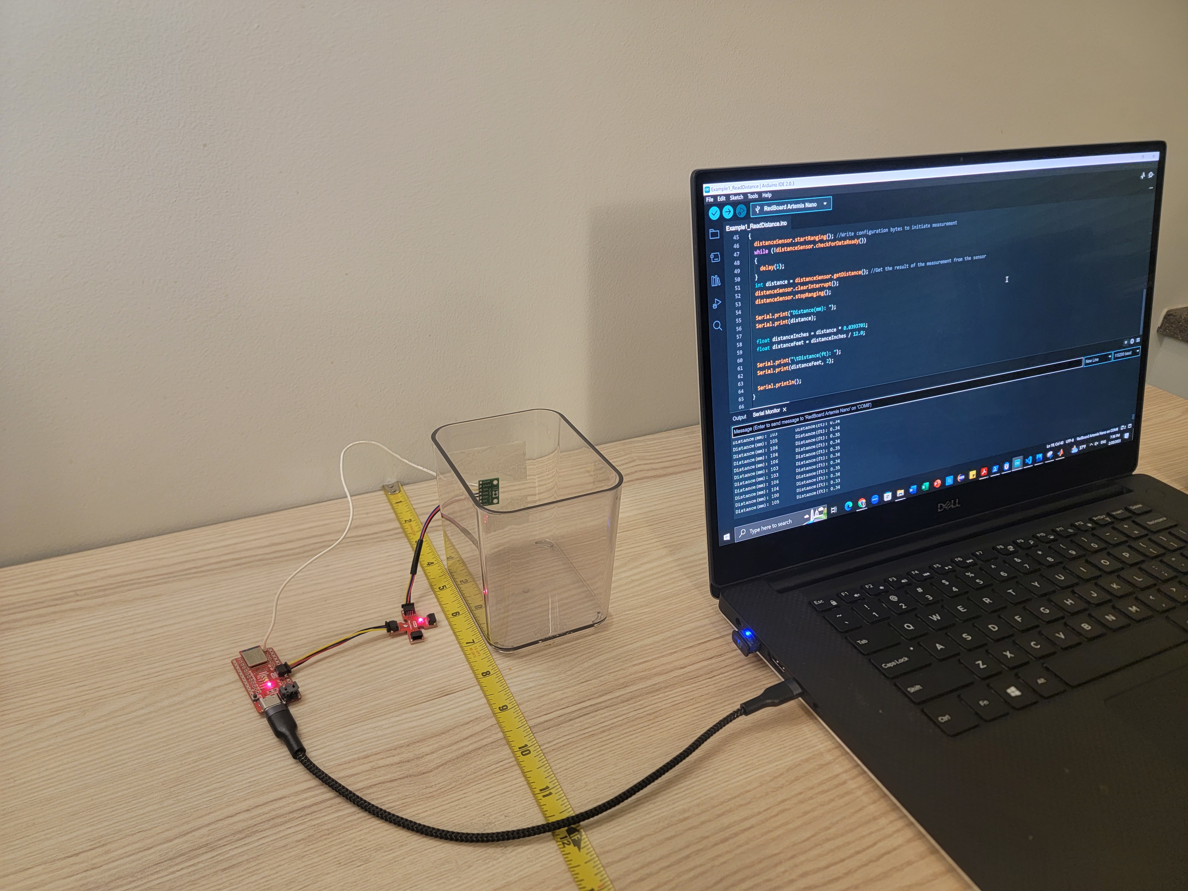
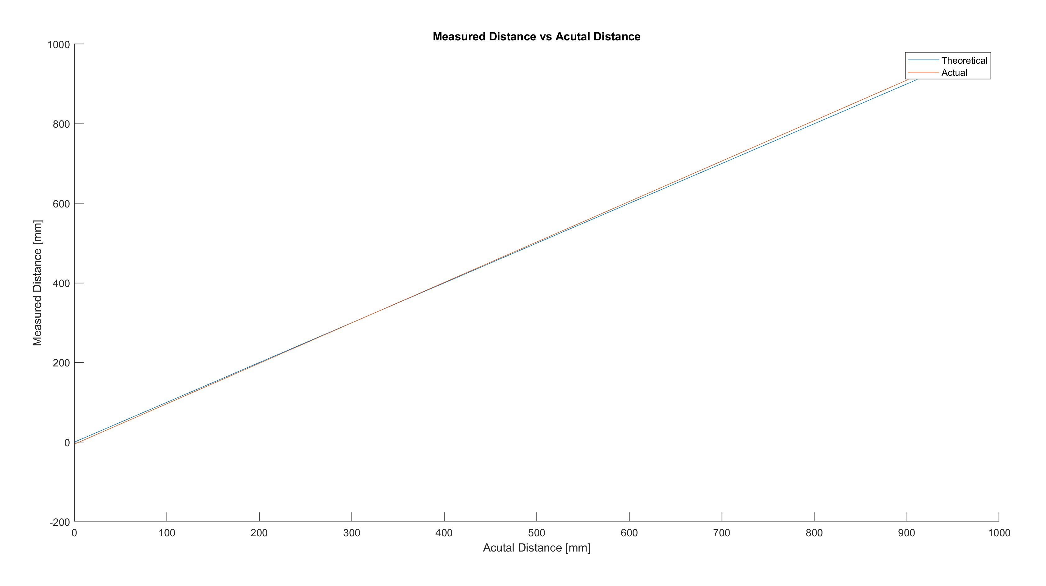
I plotted the measured distance vs actual distance in MATLAB. From this, I observed that the error between the measured distance and actual distance increases as we go further in distance.
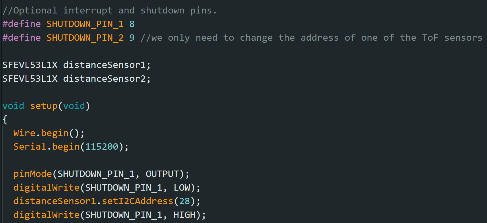
I hooked up both ToF sensors simultaneously and utilized the shutdown pin to change the address of one of the ToF sensors. I left one of the address as default, 52, and changed the other address to my number of choice, 28.
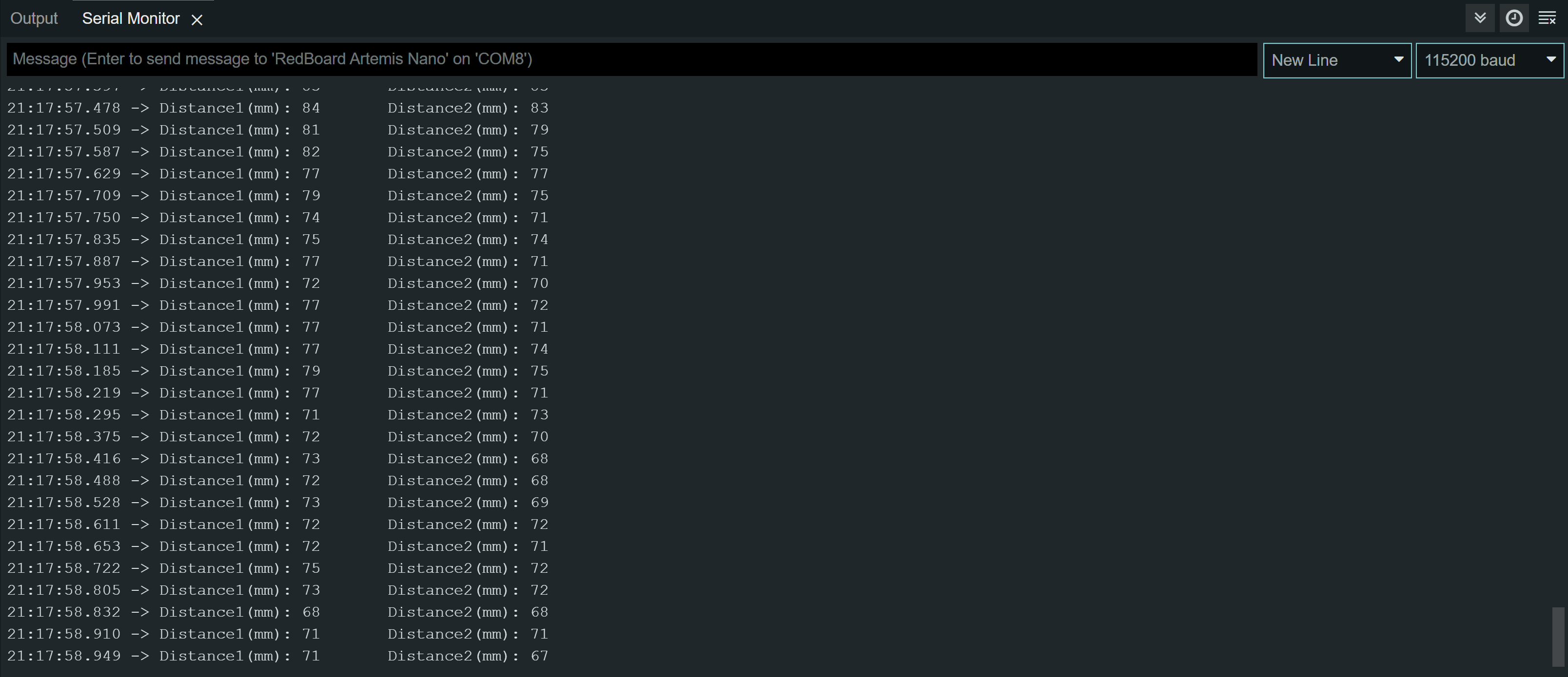
From doing so, I was able to get both distance readings from the two ToF sensors.
I want the code execute quickly, without waiting for the sensors to finish measurements. So, I coded the Artermis to print the Artemis clock to the Serial continuously, as fast as possible, while only printing the new ToF sensor data from both sensors when they are available.
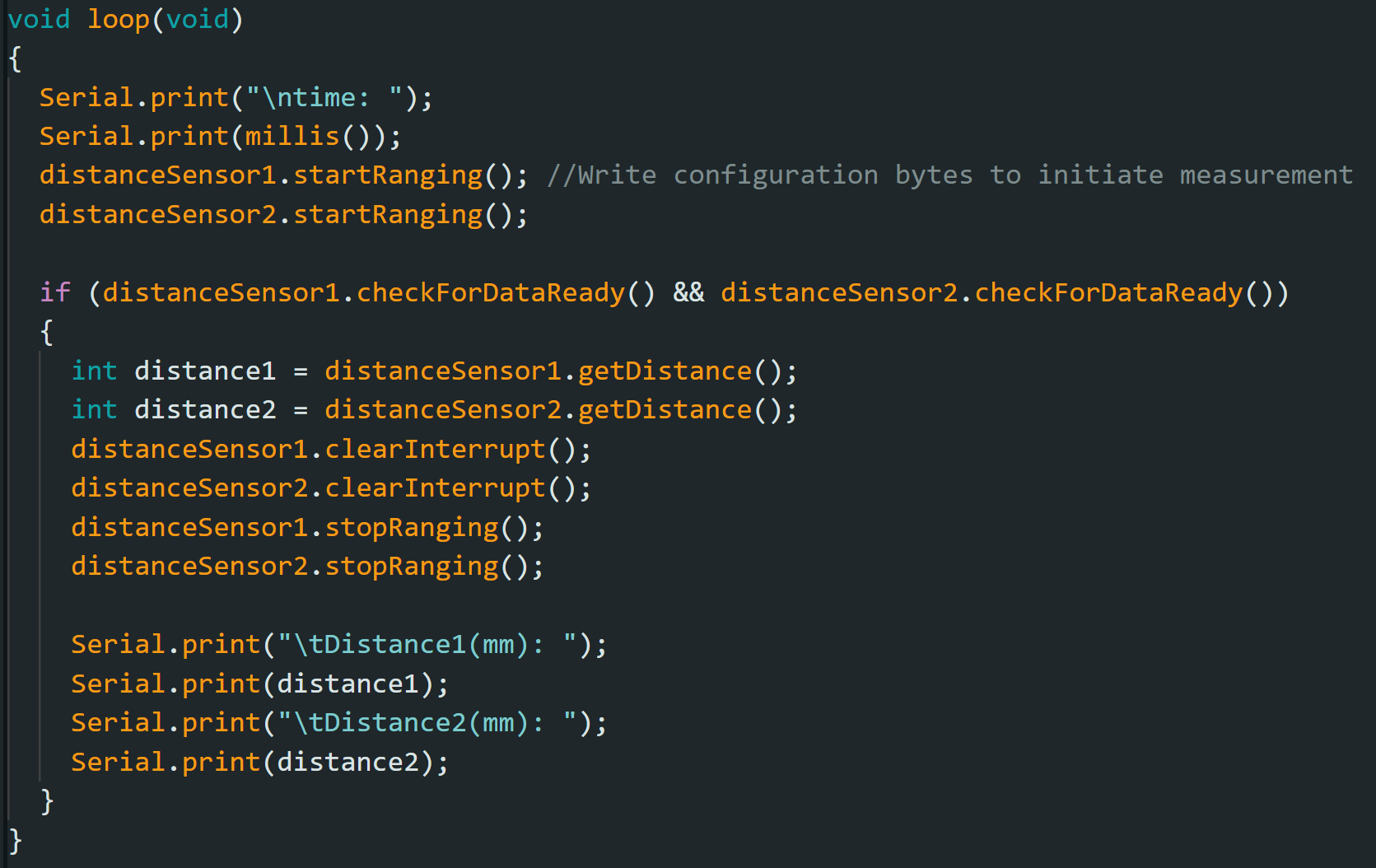
My loop executes at about 62 milliseconds. The current limiting factor is the run time of my checkForDataReady(). Whenever new data is available, I can send that data to the serial.
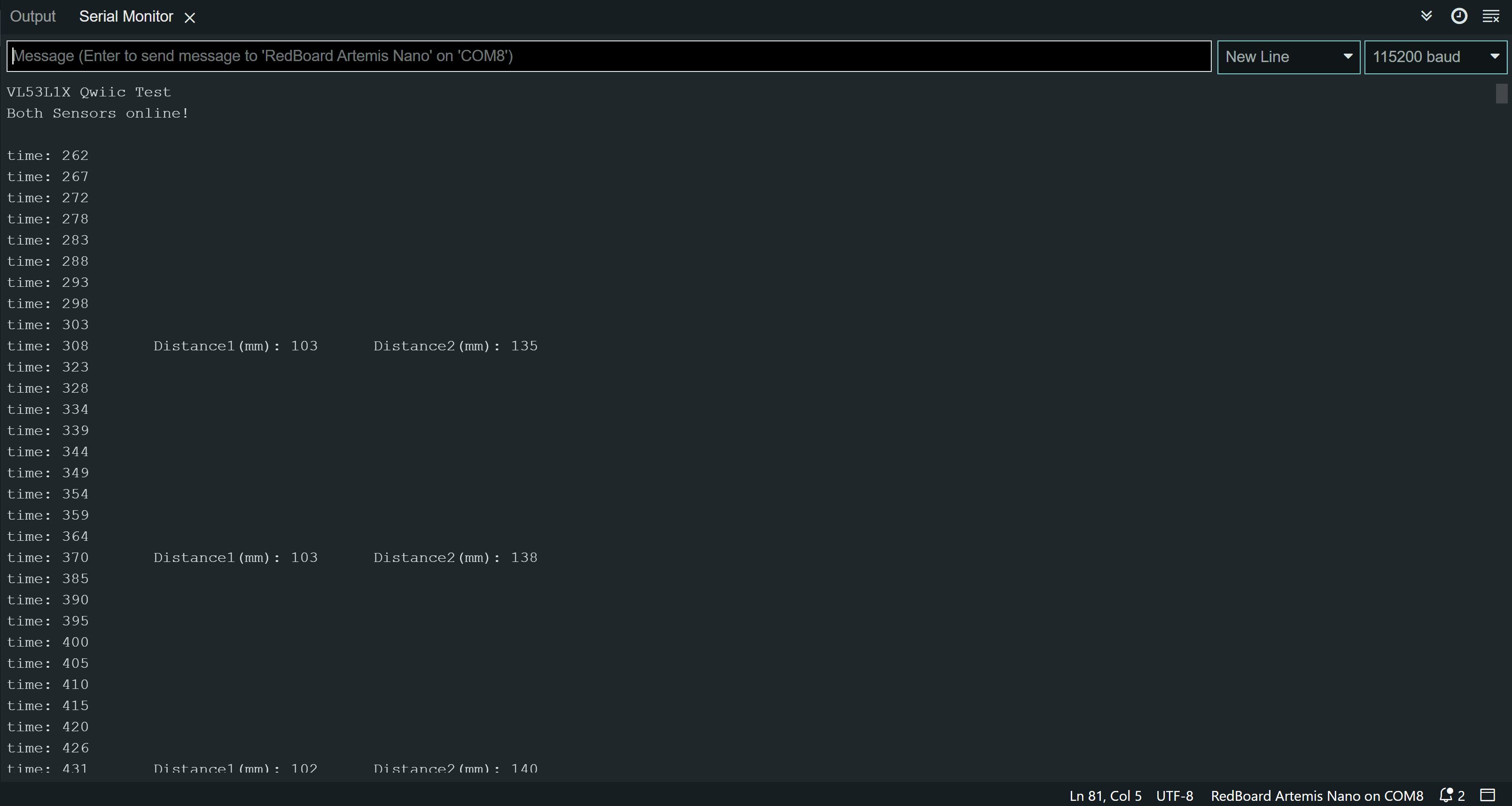
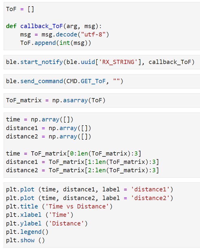
I added to my work from lab 2 so that I can record time-stamped ToF data for a set period of time and send it over Bluetooth.
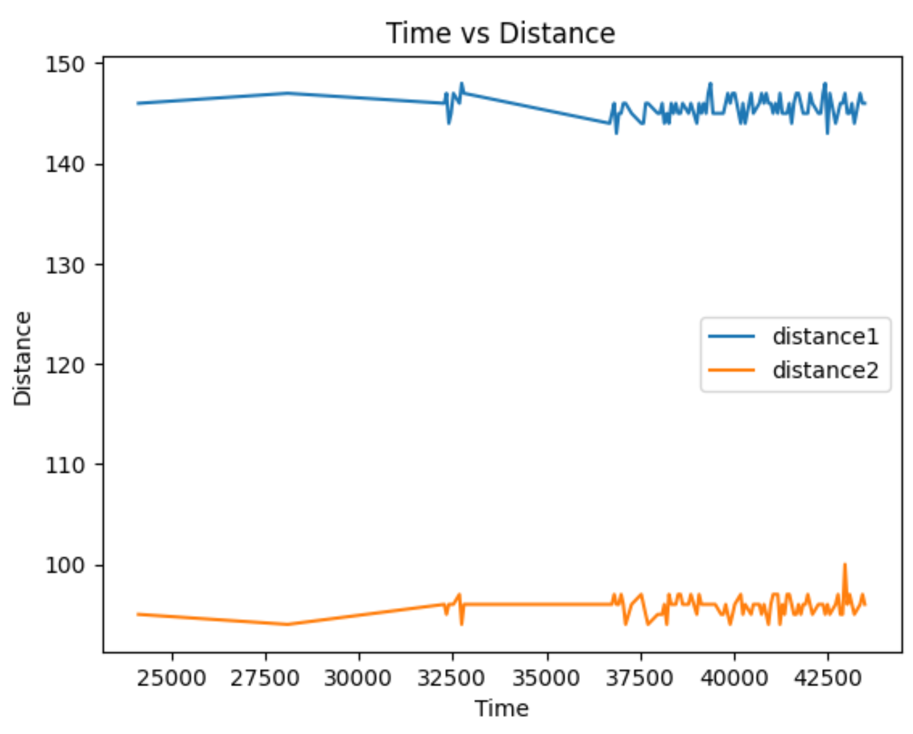
Below is a time vs distance graph, generated by Artemis clock data and both of my sensor data.
The goal of this lab is to be able to use the IMU sensor on the robot and start running the artemis from a battery.
The IMU I used in this lab is the SparkFun 9DoF IMU Breakout - ICM-20948 (Qwiic) board. I read upon the software library and the datasheet to prepare for the lab.
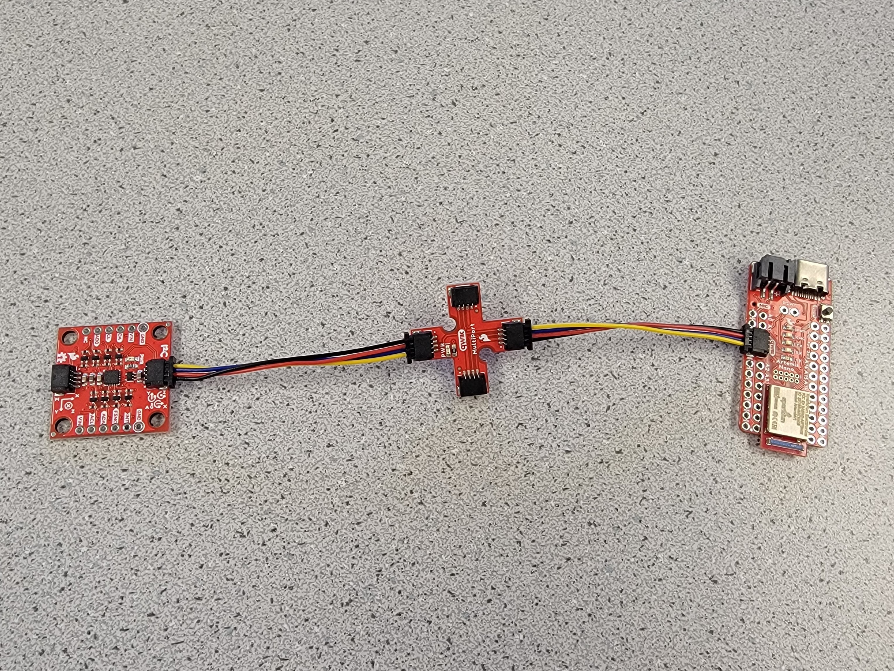
The picture below shows my Artemis IMU connections. The IMU is connected to the Artemis board using the QWIIC connectors.
I installed the SparkFun 9DOF IMU Breakout - ICM 20948 - Arduino Library. Then, I uploaded the code found from "File->Examples->SparkFun 9DoF IMU Breakout - ICM 20948 - Arduino library->Arduino->Example1_Basics" to check that the IMU example code works.
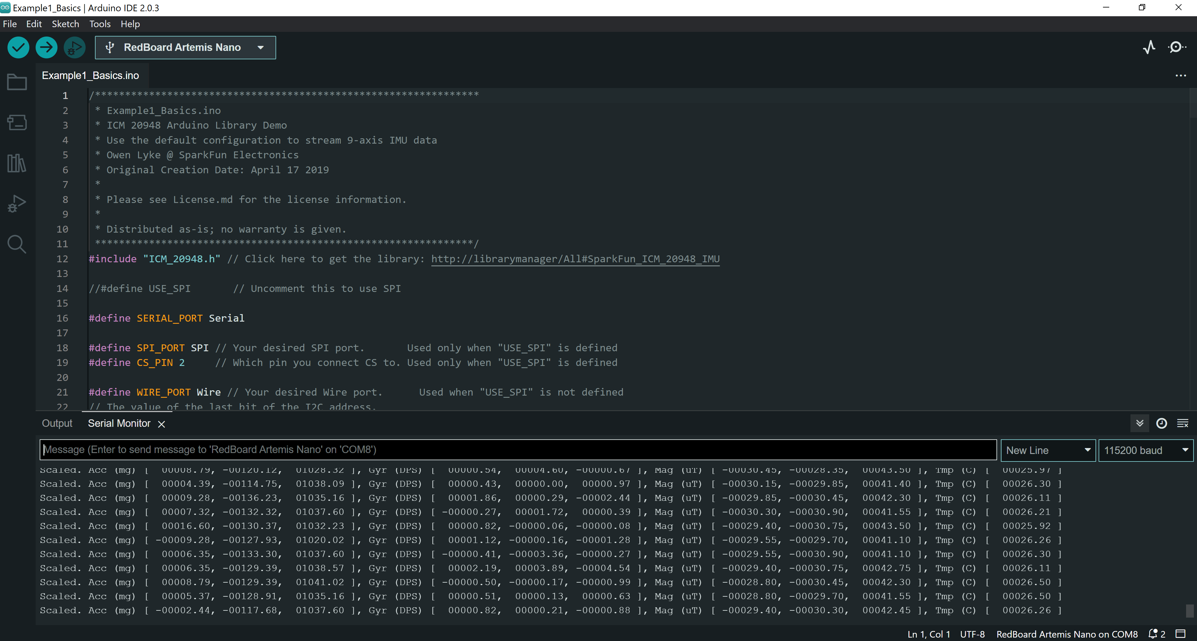
AD0_VAL is the value of the last bit of the I2C address. By default, the bridge of the ADR on I2C board is not connected, and the corresponding default value on the SparkFun 9DoF IMU breakout is 1. When the ADR jumper bridge is connected, the value becomes 0. Since I didn't connect any bridges, I set ADO_VAL to the default value of 1.
In order to have a visual indication that my board is running, I added code to blink the LED on Arthemis at the end of the setup.

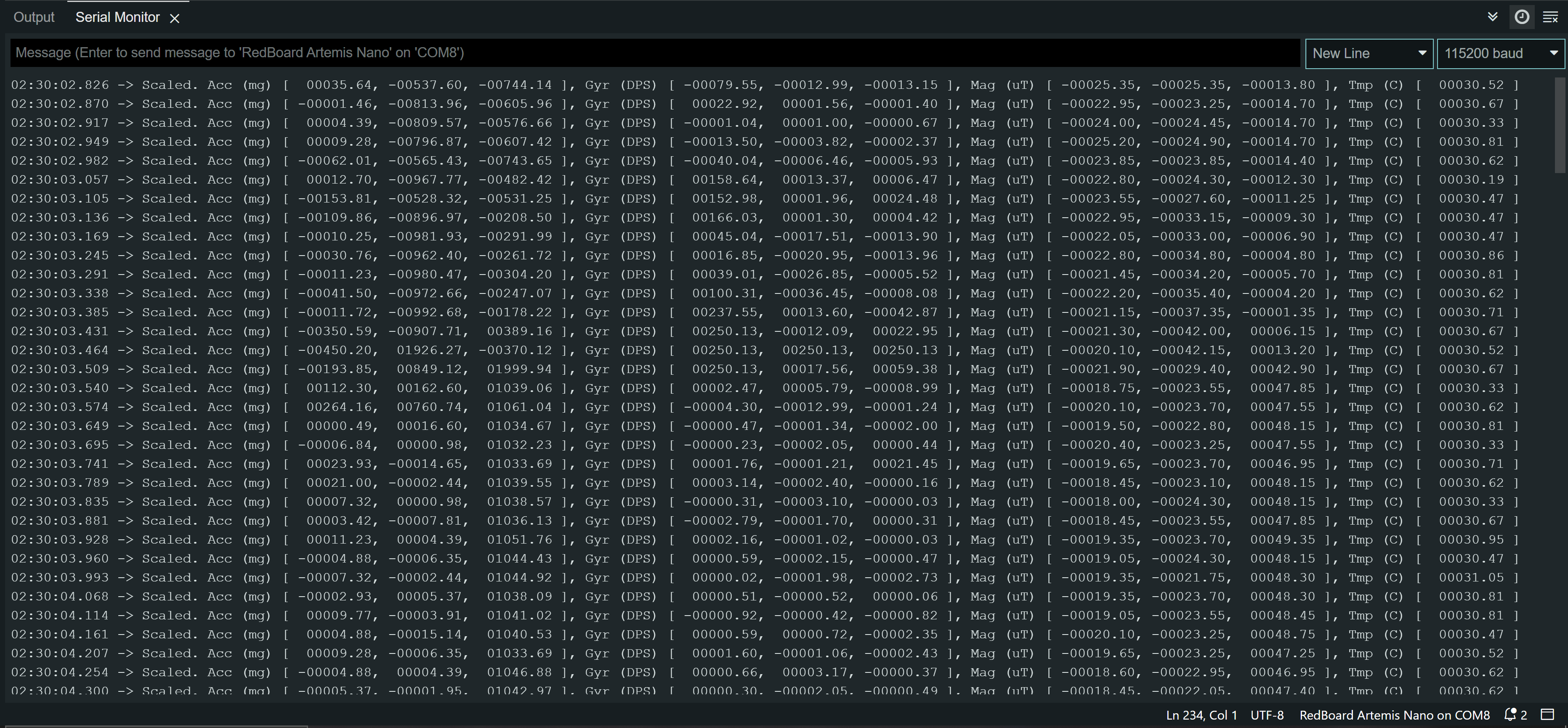
In the serial monitor, both acceleration and gyroscope data for x,y, and z was shown. I observed that the sensor values change as I rotate, flip, and accelerate the board. When I rotate the board, the gyroscope data changed. When I accelerated the board, I saw that the accerleration data changed.
Based on the equations from class, I converted the accelerometer data from the IMU into pitch and roll.

I used the surface of the table as a guide to check my pitcha and roll output when I rotate my IMU -90, 0 and 90 degrees. By doing so, I observed that the accelerometer seems pretty accurate with uncertainty of 4 degrees in pitch and roll.
I recorded my accelerometer data to analyze the noise in the frequency spectrum. I followed the guidelines from here to do a Fourier Transform in Python. Below are my graphs for time vs pitch, time vs roll, frequency domain signal for pitch, and frequency domain signal for roll.
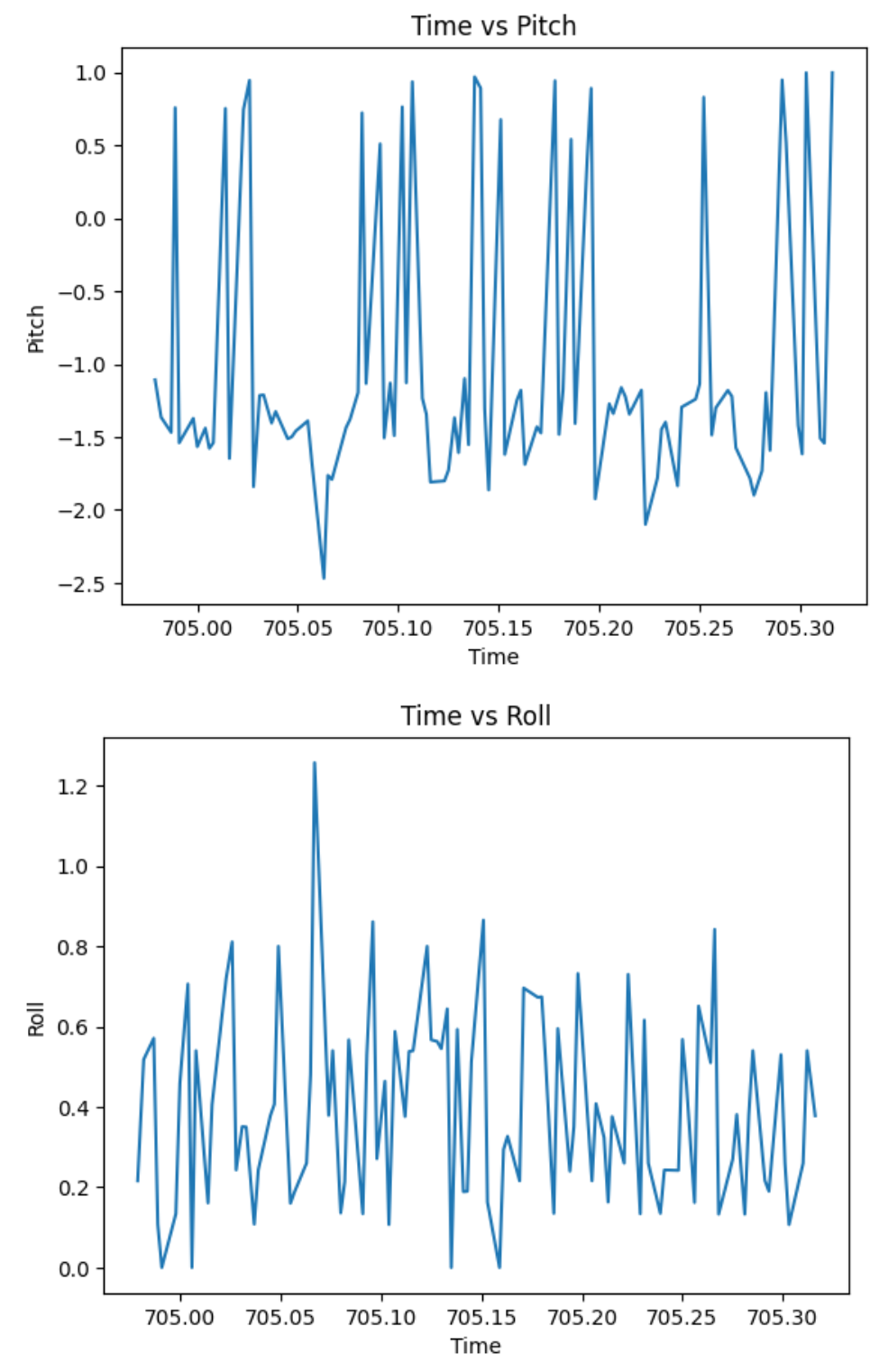
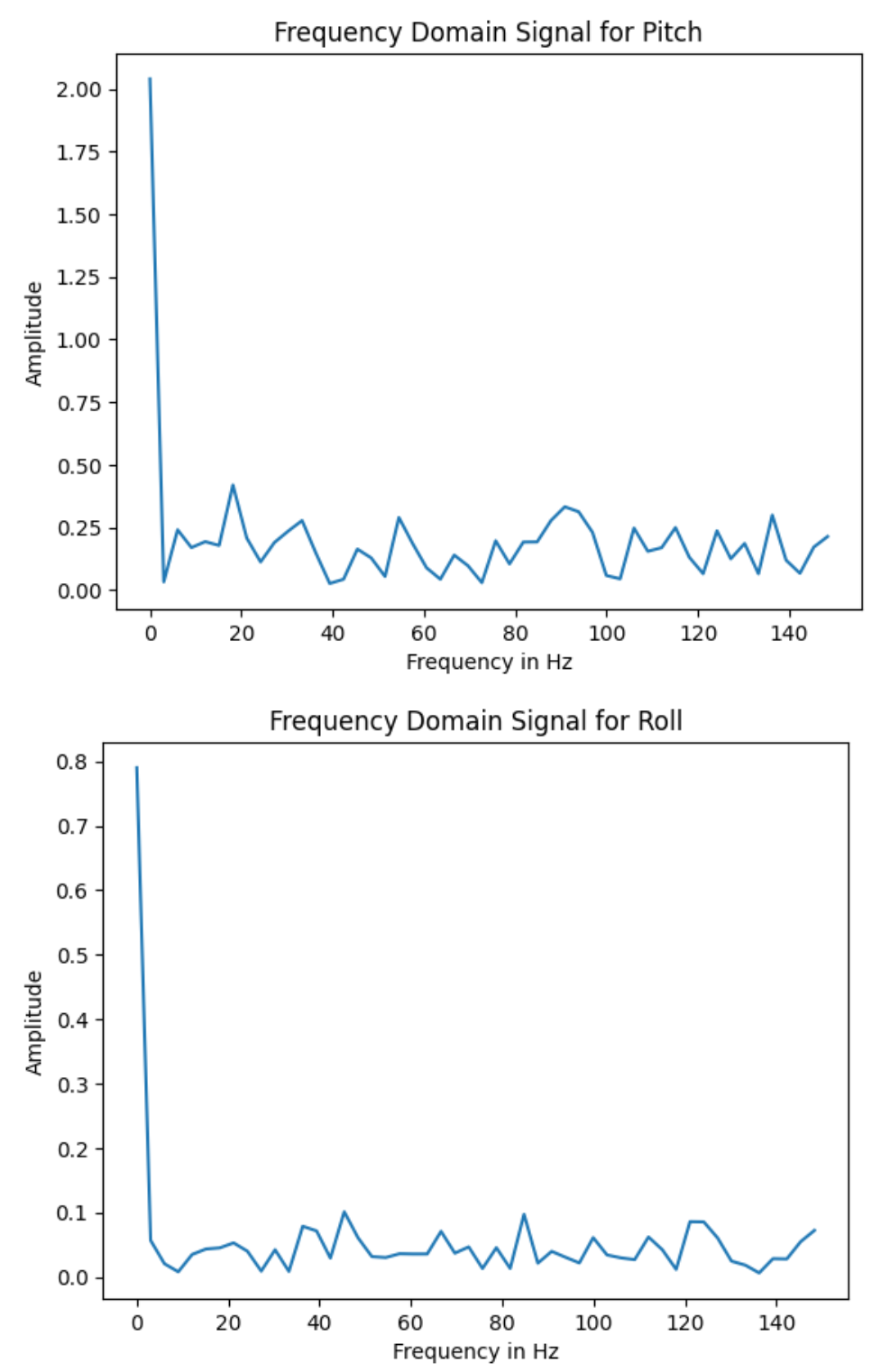
As shown in the graphs above, there is very little noise. This may be because my chip's built-in low pass filter is activated by default. Since the data is already low-pass filtered, I will not add an additional low pass filter.
Based on the equations from class, I converted the gyroscope data into pitch, roll, and yaw angles.
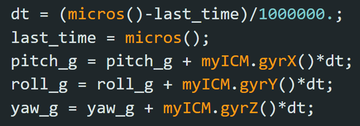
Gyroscope's pitch, roll, and yaw angles seems like they drift more, but have lower noise, compared to accelerometer's pitch and roll. This is shown in video below. In addition, I observed that increasing the samping frequency makes my accelerometer and gyroscope data match more similarly. The video shows the gyroscope's pitch, roll, and yaw, as well as accelerometer's pitch and roll.
I combined gyroscope's data and accelerometer's data to create a complimentary fliter.

The complimentary filtered pitch and roll data looks more both accurate and stable. In addition, it is more immune to drift and quick vibrations. The video shows the complimentary filtered pitch and roll data.
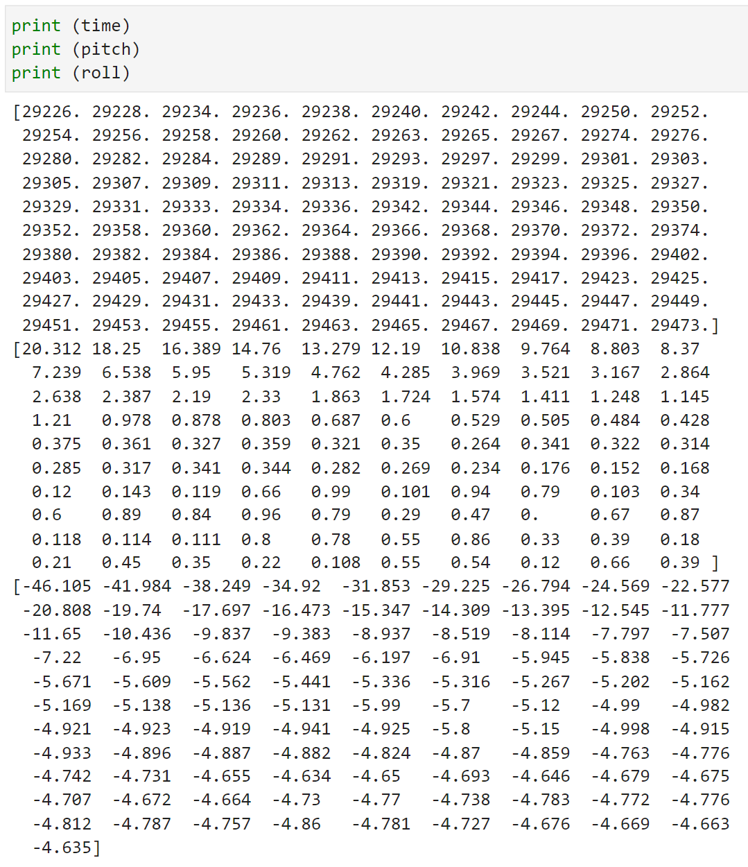
Similar to Lab 3, I don't the wait for the IMU data to be ready. Instead, I check if data is ready in every iteration of the main loop and store that value. I removed any delays and Serial.print statements in my ardunio code to reduce delays. Below is my stored time-stamped IMU data in 3 arrays: time, pitch, and roll. By looking at the increments in the time stamp, I oberserved that I am able to sample data about every two milliseconds.
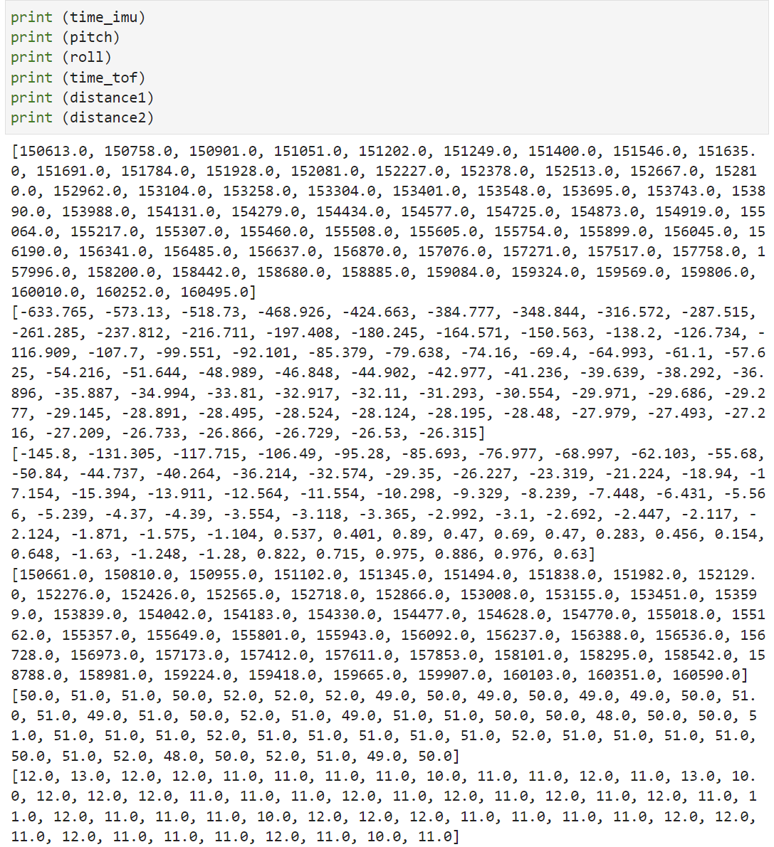
I integrated my code from lab 3 so that the Artemis captures both IMU data and ToF data. I decided to divide up the array to check if my ICM data is ready and if my distance sensor data is ready separately so that I don't waste time waiting for both things to be ready. I send my complimentary filtered pitch and roll data, which integrates my accelerometer and gyroscope data, and my distance sensor data, along with their corresponding time stamps, over bluetooth for 10 seconds.
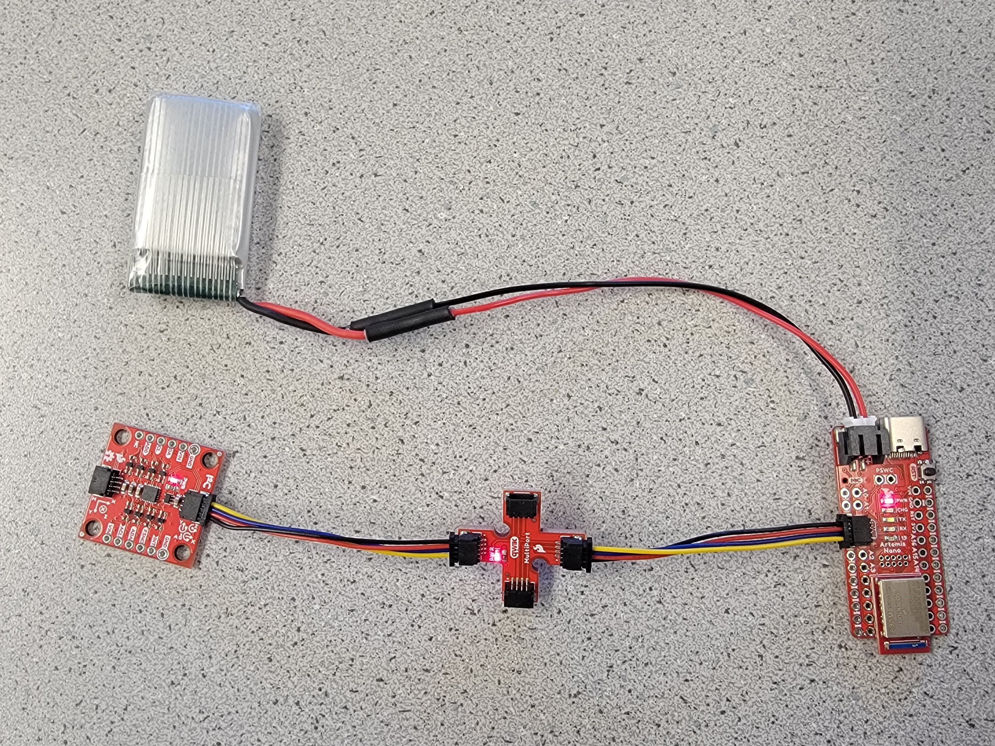
There are two types of batteries: 3.7V 850mAh and 3.7V 650mAh. I chose to use the 3.7V 850mAh battery to power the motors and the 3.7V 650mAh battery to power the digital electronics. I chose to use the battery with more capacity to drive the motors because the motors will use up the battery more quickly. Below is a picture of my Artemis connected to the 650mAh battery:
I mounted the 850mAh battery to the car. Then, I drove the car around with the controller to get a feel of how fast the car drives and turns. Below is a video of the car being driven without the artemis board. I tried to do flips and spins with the car.
Below is a video of the car doing flips with the artemis board, the IMU, and the distance sensors.
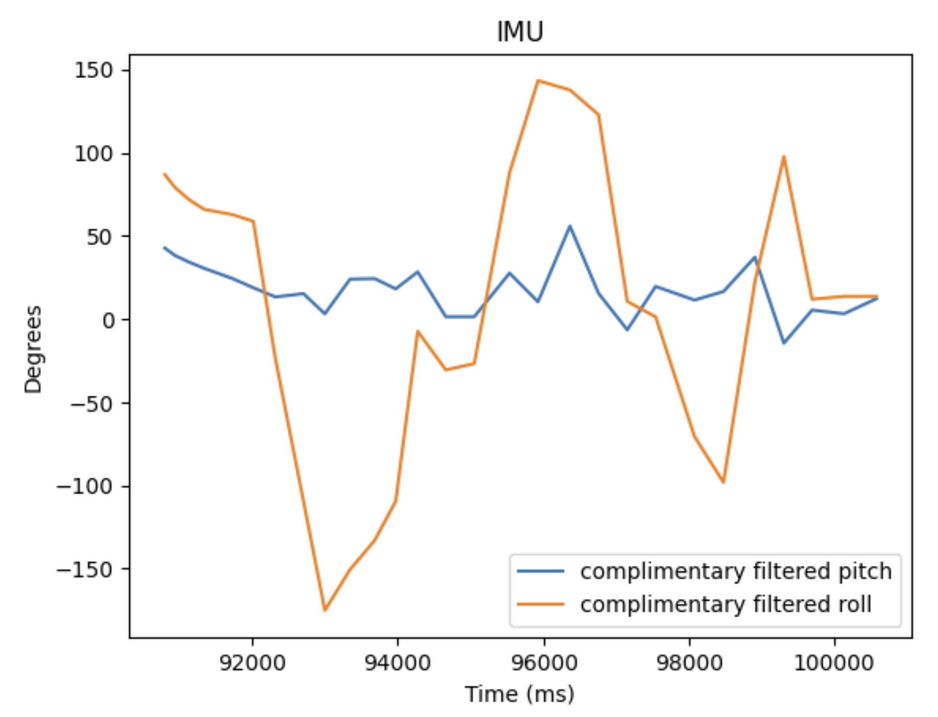
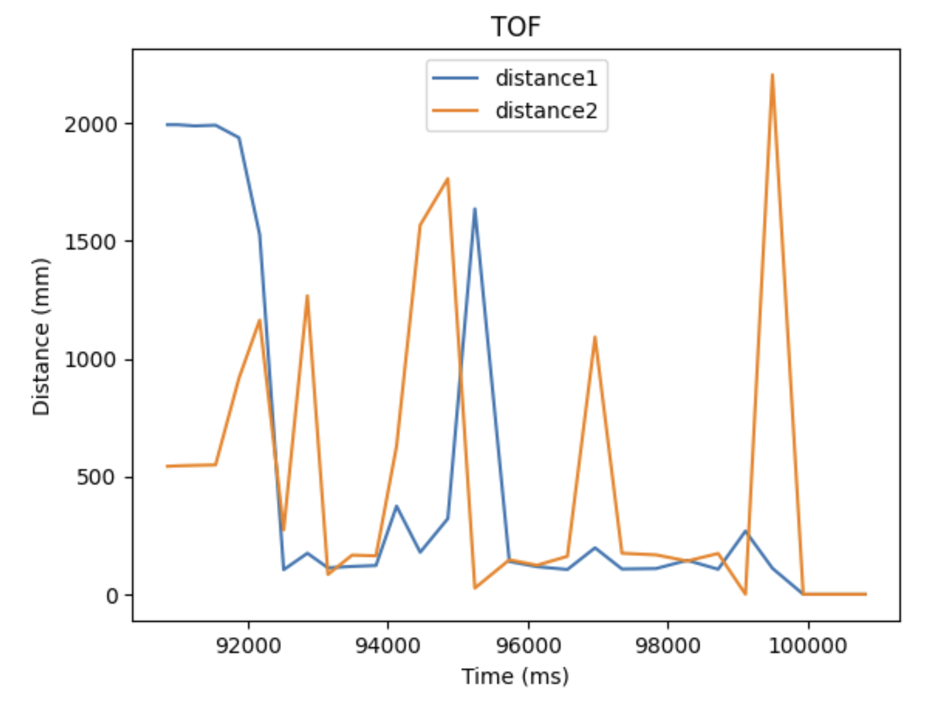
I recorded both the IMU data and ToF data over bluetooth for 10 seconds while doing flips shown in the video above. Below are my plots of the IMU data and the ToF data.
The goal of this lab was to be able to control the motor drivers with the Artemis, as well as fully integrate the car's chassis with all the electrical components.
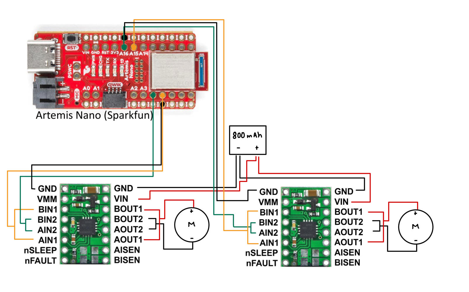
I parallel-coupled the two inputs and the outputs of the dual motor drivers to deliver double the current without overheating the chip. I decided to use pins 4, A5, A15, and A16 on the Artemis to send PWM signals to the motors. Since long wires may lead to unnecessary noise, I tried make the wires just the right length. I decided to power the Artemis and the motor drivers/motors from separate batteries, and I also placed the sensors farer way from the motors inorder to reduce noise.
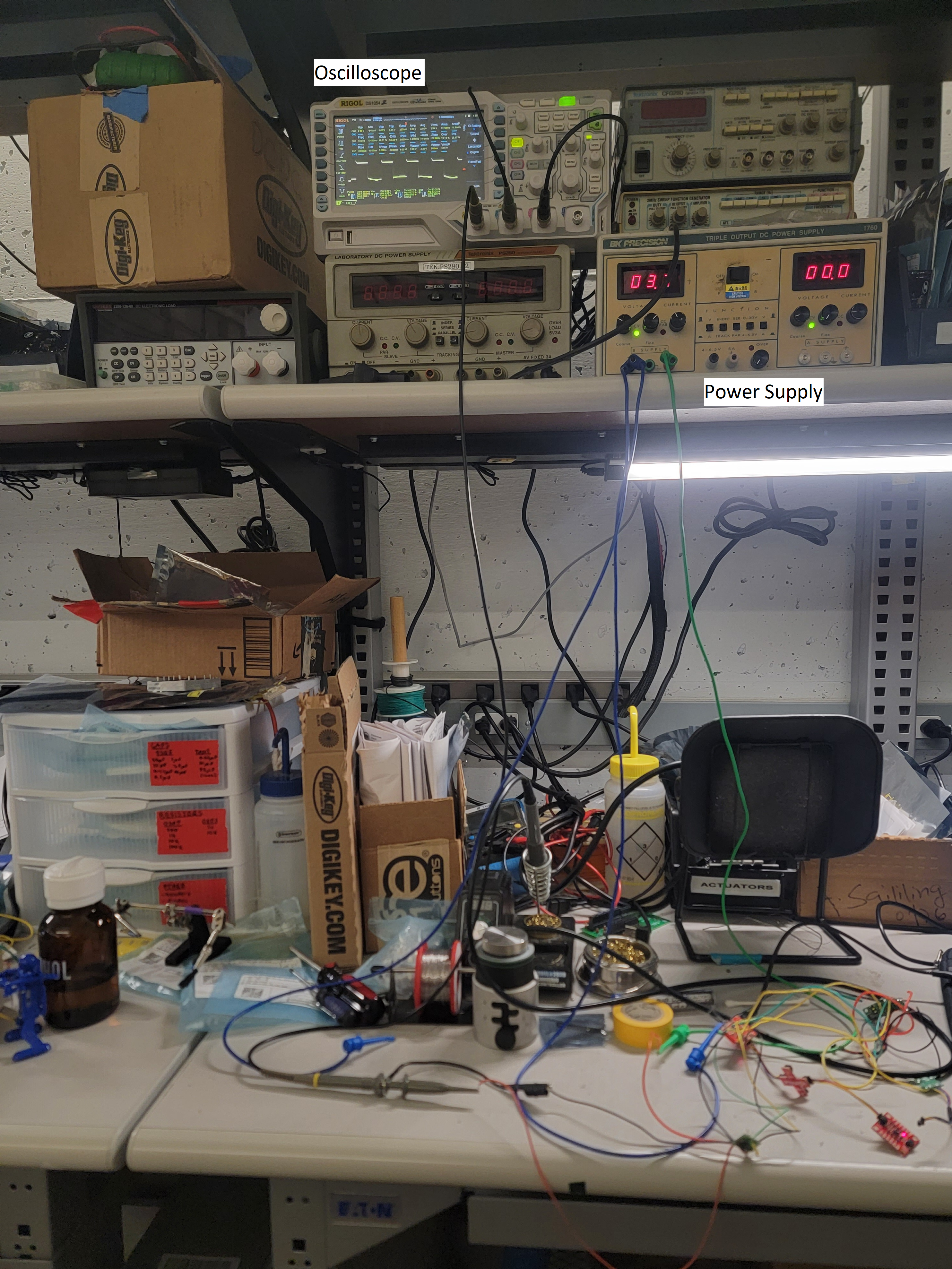
I connected the motor driver (VIN) to the external power supply to test if my circuity is correct and that I can regulate the power on the motor driver output. I set the input voltage to 3.7V inorder to replicate the voltage of the motor batteries.
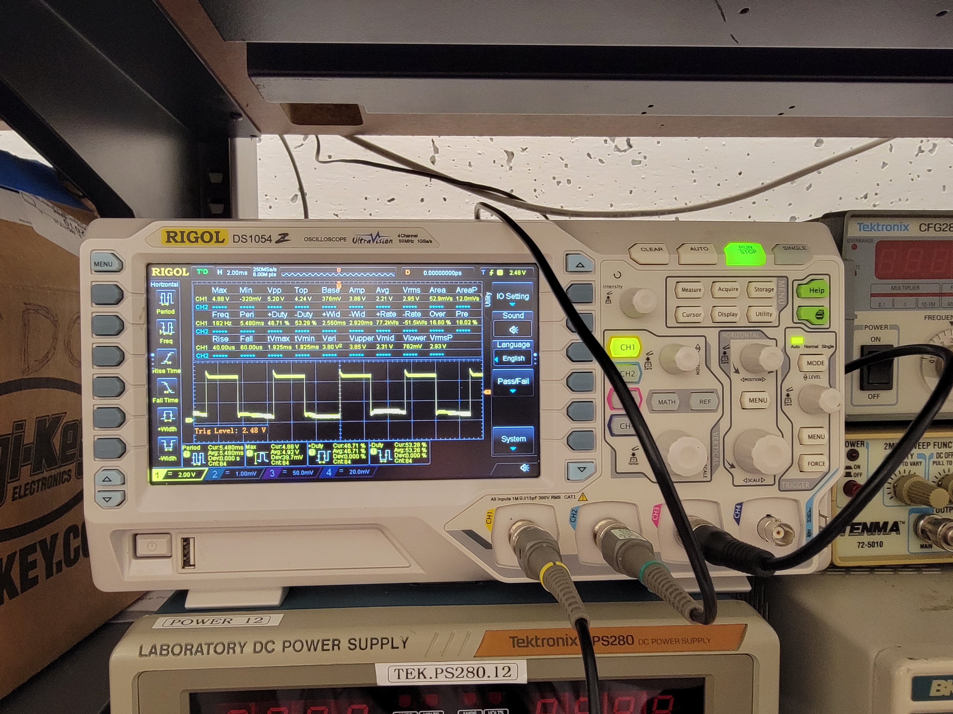
I used the analogWrite() command to generate PWM signals to the motor driver. The oscilloscope verifies that the connections are corrects and shows my PWM signal. Below is my code snippet to generate the PWN signal shown in the oscilloscope.
Now that I verified that my wiring is correct, I soldered both motor drivers to the battery connectors. Below are videos of the motor drivers being tested.
One motor spinning forward:
One motor spinning backward:
Both motors spinning forward:
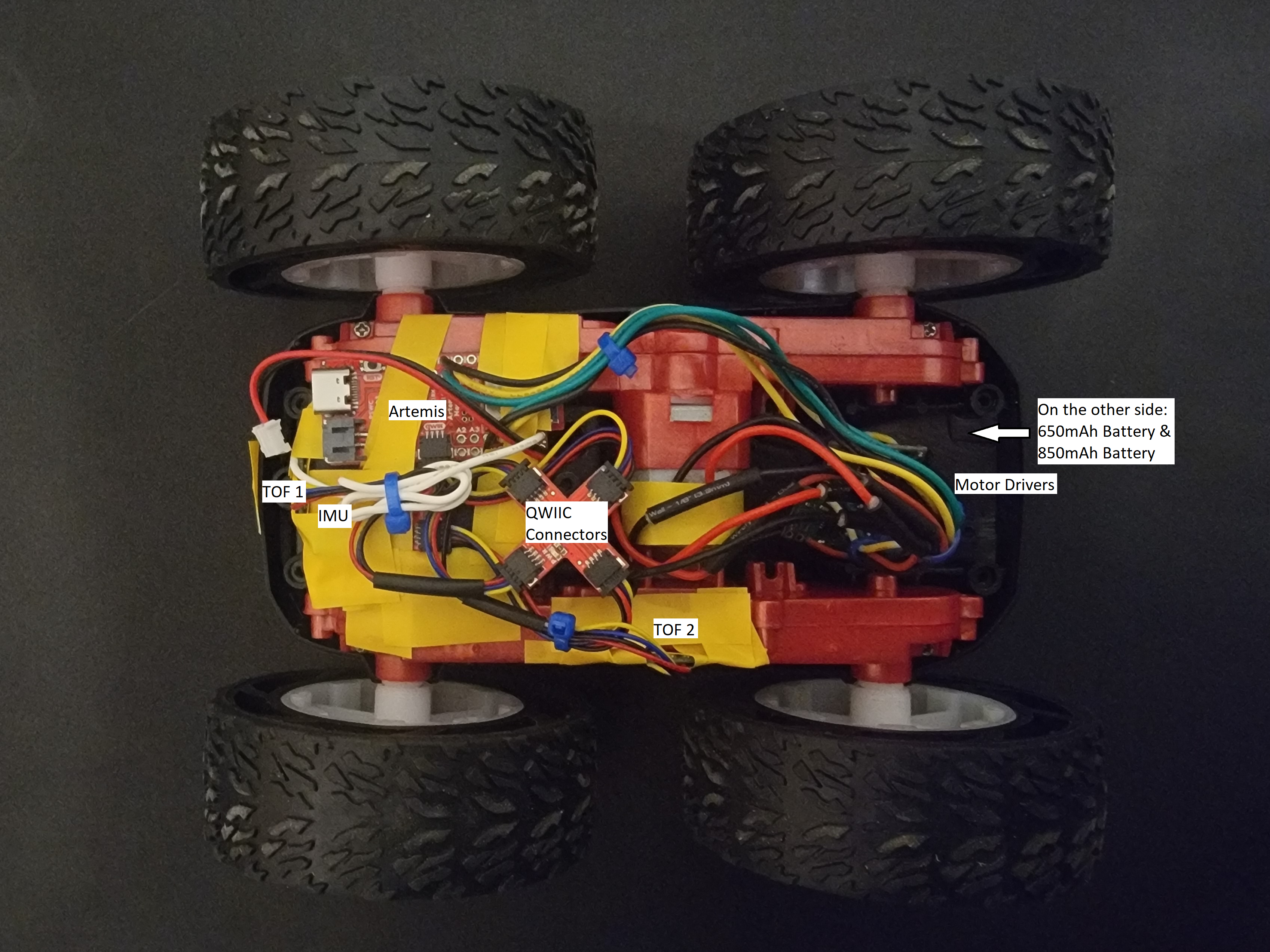
Below is a picture of my car, fully assembled with the Artemis, IMU, 2 TOF sensors, 2 motor drivers, 2 motors, QWIIC connectors, 650mAh battery and the 850mAh battery. I secured one TOF sensor to the front of the car and and the other to the left of the car. I tried to put the IMU away from the motors to reduce noise as well as flat on top of the car so that the pitch and yall data are easy to interpret. In addition, I put both of the batteries in the battery compartment of the car.
By slowly increasing the PWM value, the lower limit of the PWM value was found to be an analogWrite() value of 40. Due to the low manufacturing quality of the motors, my car was drifting left when I assign the same analogWrite() values to both of the motors. The video shows how my car behaves without any calibration.
I calibrated the motors so that the left motor spins faster than the right motor. Below is a video of my car driving straight for about 8 ft. My calibration code snippet is also shown below.
Below is my demonstration of open loop control. I tried to go forward, left, forward, right, and backward.
The goal of this lab to use a proportional controller to drive my car as fast as possible towards a wall and stop exactly 1ft (304 mm) away from the wall.
For the prelab, I decided to set up a system so that my robot can start from an input from my computer, sent over Bluetooth. Below is my structure for the command types.
In addition, I made ardunio take in input values from the computer to set values such as the motor input or the Kp value to make testing easiler. Below is my code snippet to handle different command types on ardunio.
For example, I can make my robot go forward with a motor input of 80, from my computer, with the command below.

PID control, which stands for proportional integral derivative control, utilizes a feedback loop to better control my car. It can help with things such as maintaing speed prediction at different battery levels and at different surfaces. Since the proportional control is the easiest to implement and in the interest of time, I decided to implement just the proportional controller. Proportional controller uses the Kp term to proportionally calculated the speed of my car based on the error between my current position and my goal position, detected my by ToF sensors. After I find the error and calcuate the new speed by multiplying Kp and the error, I store that information in an array. After I log all of my data, I send it over to my computer via bluetooth. Below is my code snippet for proportional control and logging data.
Since my robot's motor controller range to actually move the robot is 45 - 255, I made a separate helper function to limit my motor input. Below is my code snippet for speed limiting.
Below is my code snippet for receive and handling data on jupyter.
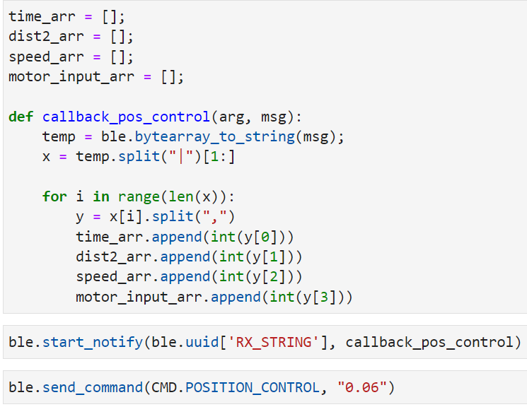
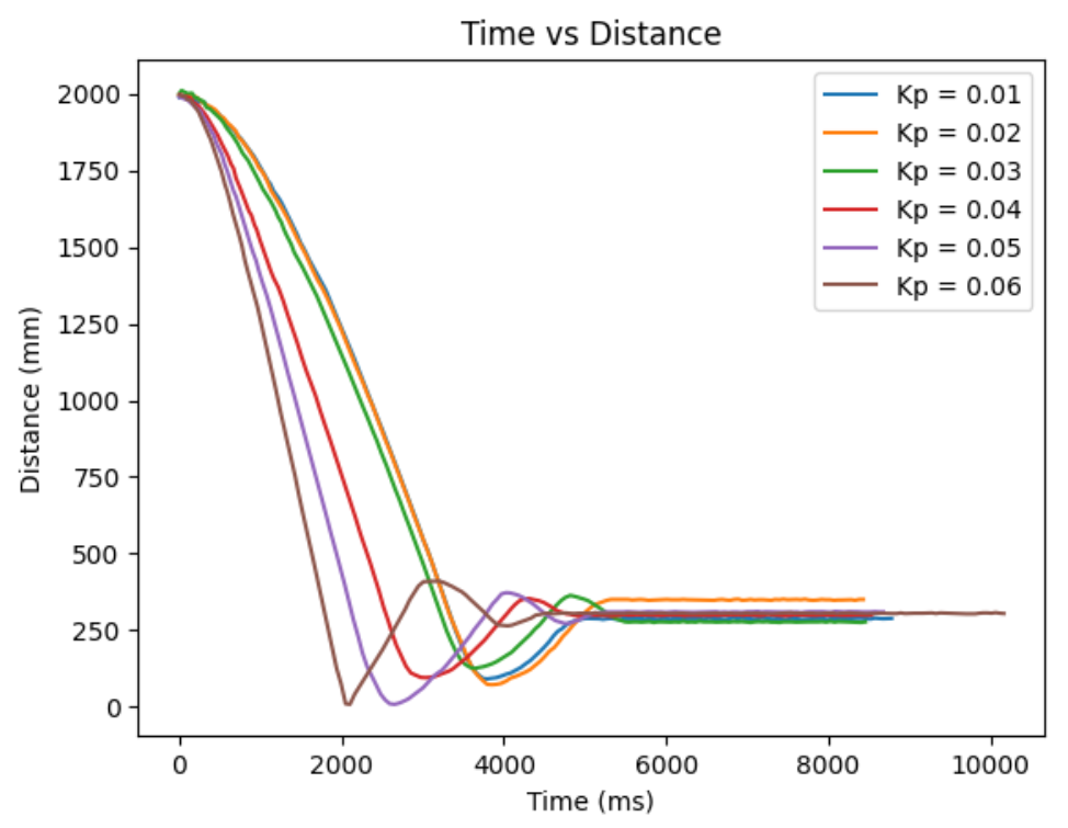
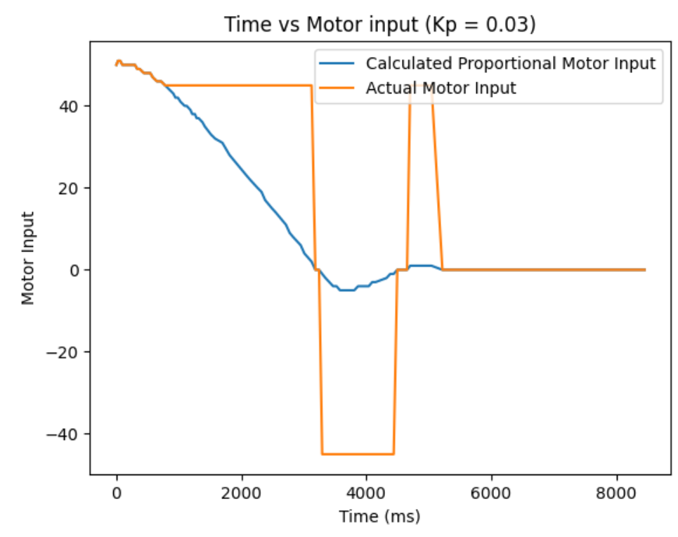
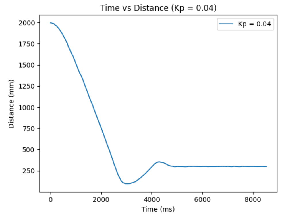
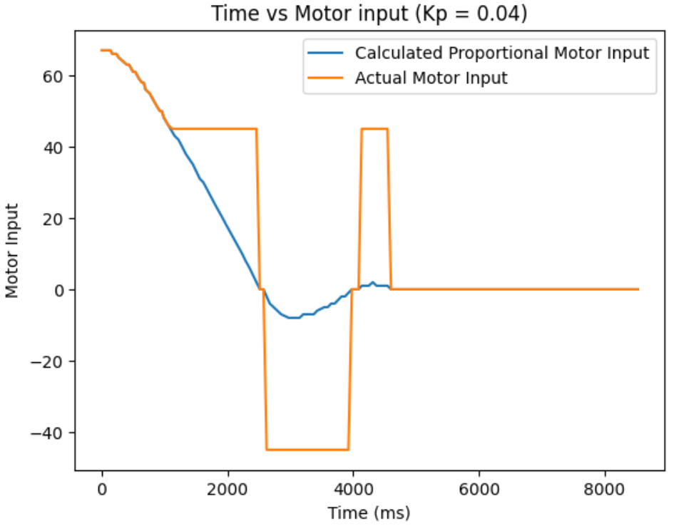
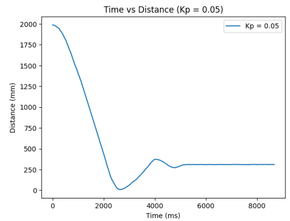
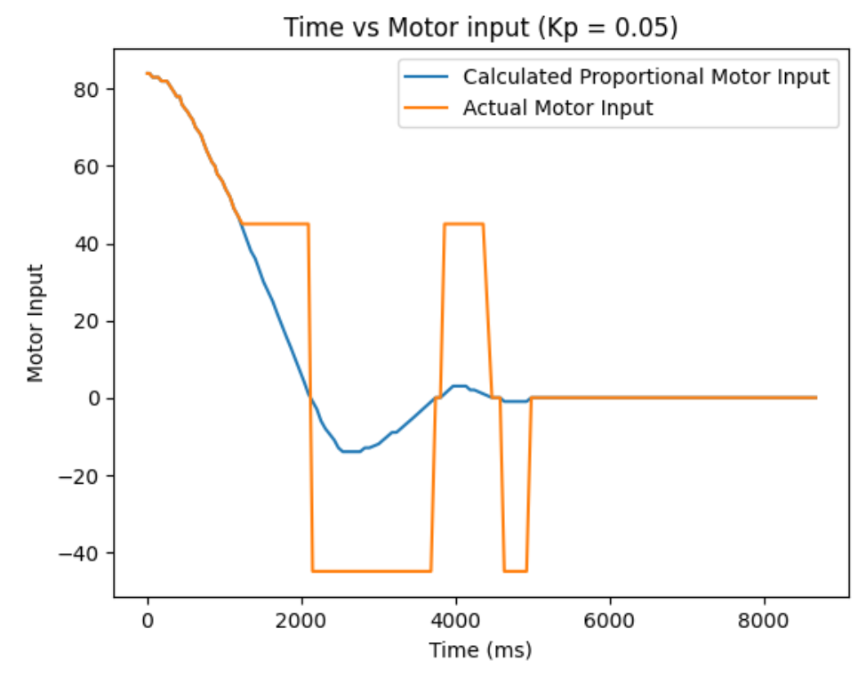
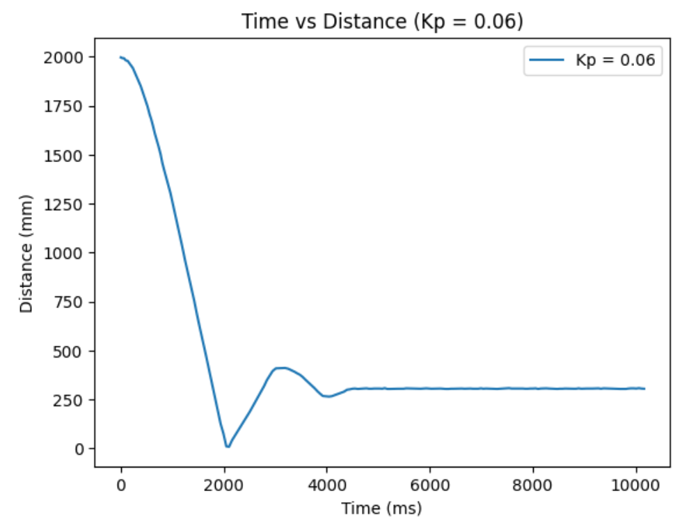
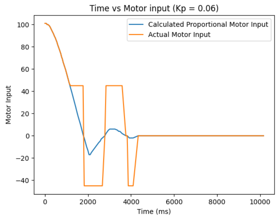
My actual range of motor input is 45-255 and the range of distance from my ToF sensor is 0-1350 mm. Based on this, I estimated that my reasonable range of proportional controller gain will be between 0.01-0.1. From actual testing, I found my robot to slightly crash at the wall when my initial distance is 2000mm from the wall and my Kp=0.06. So, I decided to record and compare my distance from the wall, proportional controller's calcuated speed input, and the actual motor input, for Kp=0.01 to Kp=0.06, with 0.01 increments. For my ToF sensor, I decided to change the sampling time. The default is 100ms, but I want more data within the time span, so I changed it to 30ms using the function setIntermeasurementPeriod();
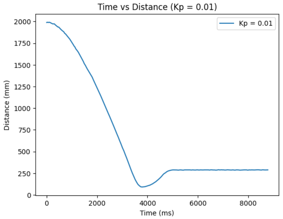
Below are my results for Kp = 0.01, 0.02, 0.03, 0.04, 0.05, and 0.06.
Kp = 0.01:
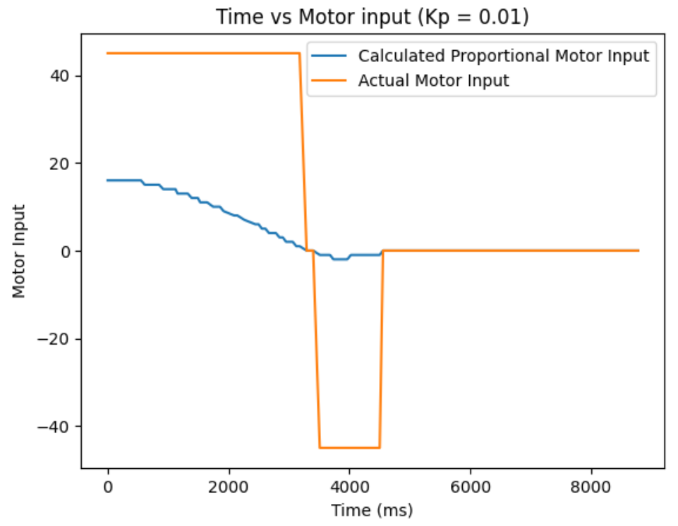
Kp = 0.02:
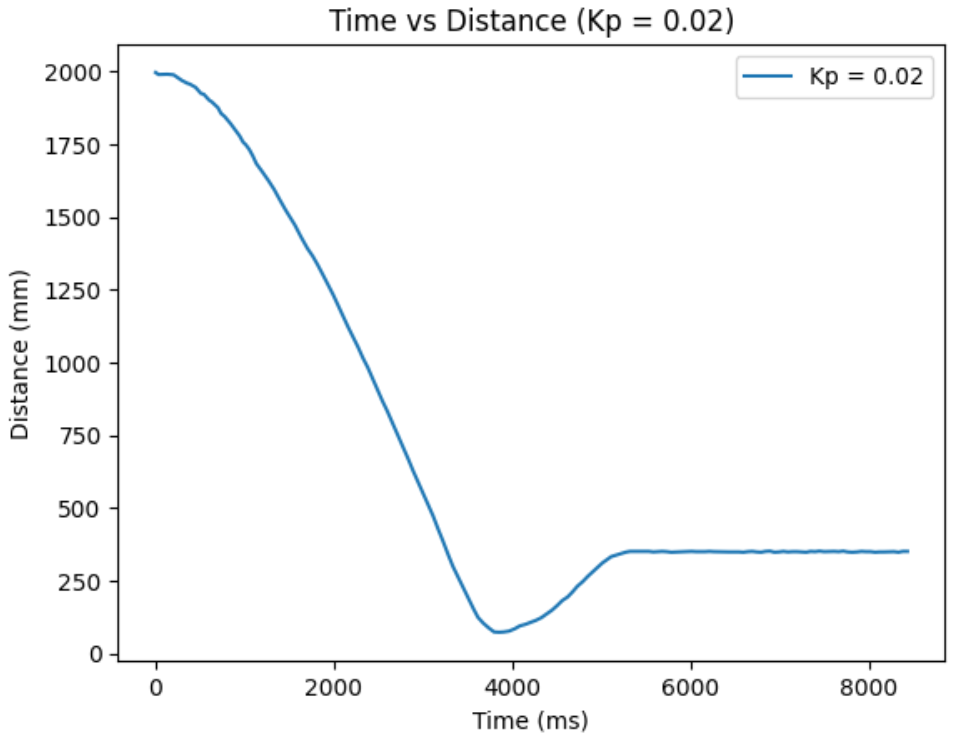
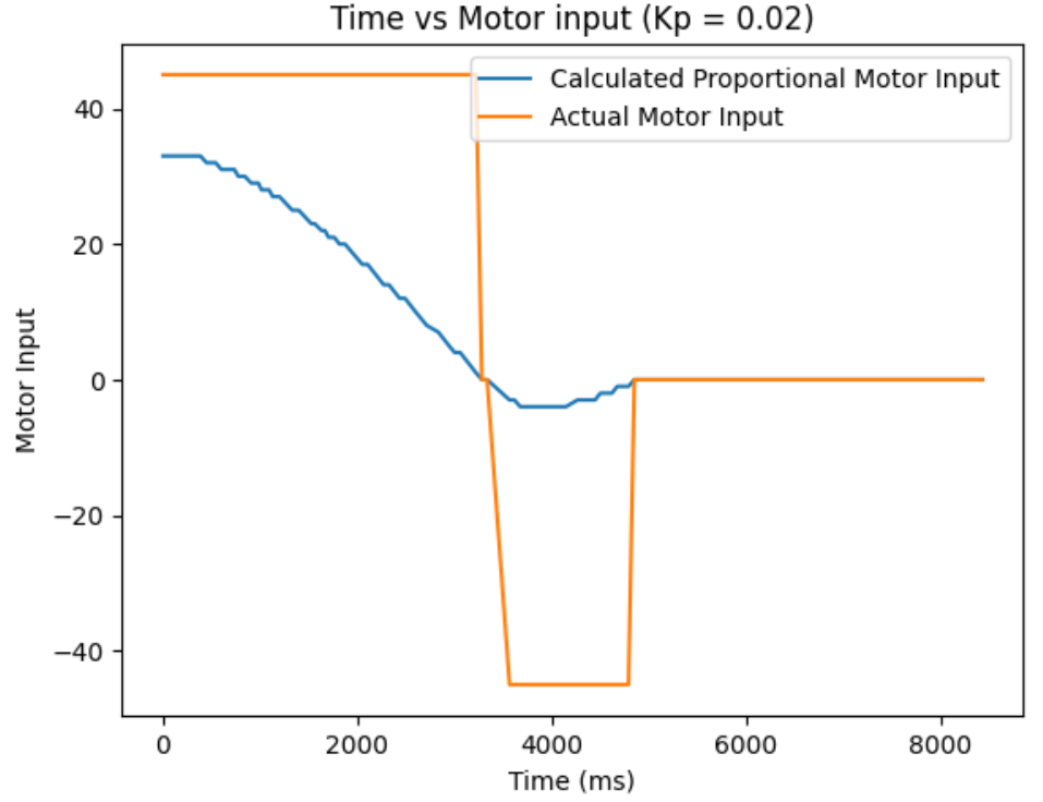
Kp = 0.03:
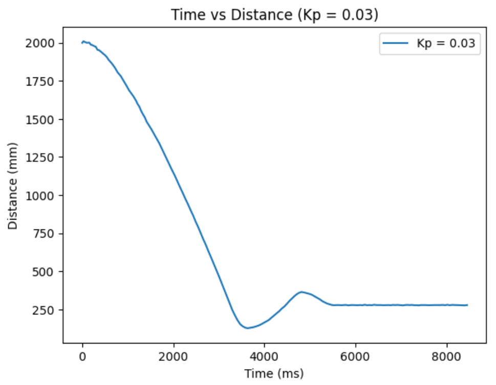
Kp = 0.04:
Kp = 0.05:
Kp = 0.06:
Combined Kp:
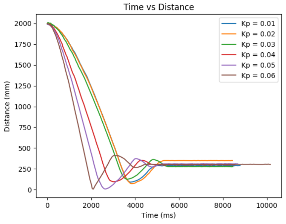
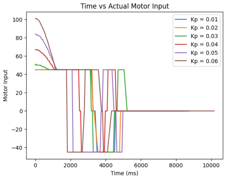
From ranging the Kp from 0.01 to 0.06, I oberserved as I increase the Kp, the more I go from having a conservative control to an aggressive control. When the Kp is too small, like when it was at Kp=0.01, the car barely overshoots and doesn't really oscillate, but it take a long time for the car to arrive even near the target distance. When the Kp is too big, like when it was at Kp=0.06, the settling time is the quickiest, but the aggresive overshoot causes the car to crash into the wall. So, I think I am the most satisfied with the results from Kp=0.04, since it had relatively quick settling time and wasn't causing my car to crash into the wall when I tested it repeatedly Kp=0.05 also had a quick settling time, but it caused my car to crash into the wall one out of three times, making it a less favorable choice.
The goal of this lab is to implement Kalman Filter in order to perform the behaviors in lab 6 faster.
State spaxe equation, as stated in the lecture, is shown below:
[ẋ; ẍ] = [0, 1; 0, -d/m][x; ẋ] + [0; 1/m]u
C = [-1, 0]
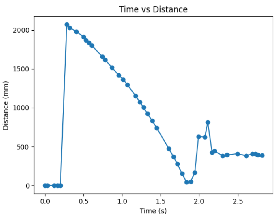
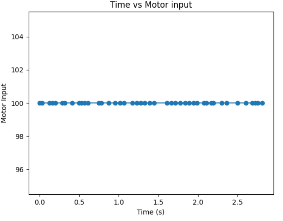
In order to build my state space model for the system, I have to estimate the drag and momentum terms for my A and B matrices. In order to do so, I drove my robot towards a wall at a constant motor input value, while logging time, distance sensor readings, and my motor input. I choose a max PWM value I used in my lab 6, which was a little bit less than 100.
Then, I created a command to go foward towards a wall for a reasonable about of time to ensure that I reach a steady state constant speed. Graphs of my data are shown below. The data after my distance reading reads zero will be thrown out since that is after my robot crashed into a wall. Reflecting on my data collection system, it would have been better to put a hard stop on the software side to avoid the mechanical damage that comes from the robot ramming into a wall.
We can manipulate the force equation to find an equation for acceleration:
F = ma = mẍ and F = u-dẋ
mẍ = u-dẋ
ẍ = (u/m)-(d/m)ẋ
At constant constant speed, ẍ is zero. So, we can find drag:
ẍ = 0 = (u/m)-(d/m)ẋ
(u)-(d)ẋ = 0
d = u/ẋ
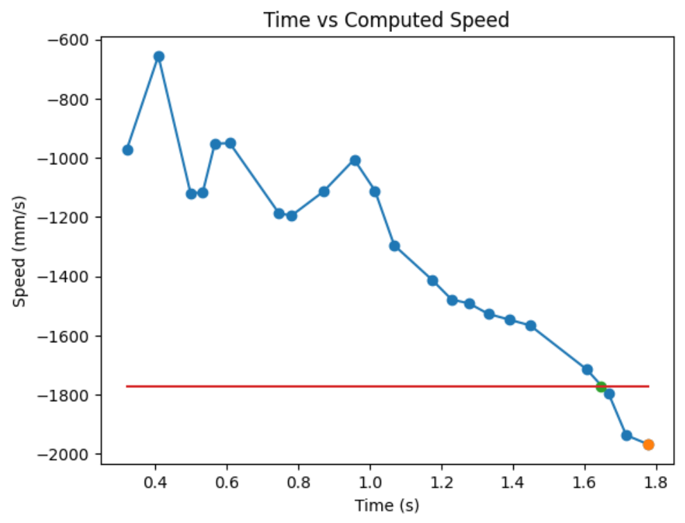
From the graph, it seems like I didn't quite make it to stedy state. Since I am very close to steady state, I will use my last derivative term, marked with an orange dot on my graph, to calculate drag. From the graph, I found ẋ to be -1966.67. Then, d = 1/1966.67mms^-1 ≈ 0.0005.
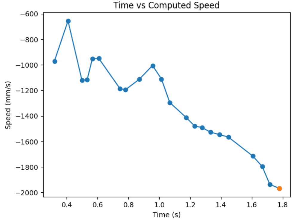
For 90% rise time, 90% of 1966.67mm/s is 1770mm/s. From the graph, I grabbed two data points near 1770mm/s and found the 90% rise time by linearly interpolating. 90% rise time = (1770-1715)/(1797-1715)*(1.666-1.607)+1.607 = 1.64657s, as shown by the green dot on the graph below. However, since my velocity slope started at 0.324sec, my actual 90% rise time is approximately 1.32657s.
Now, I can use my rise time to find m.
v̇ = (u/m) - (d/m)v
v = 1 - e^((-d/m)*t_0.9)
1-v = e^((-d/m)*t_0.9)
ln(1-v) = (d/m)*t_0.9
m = (-d*t_0.9)/(ln(1-0.9))
When I plug in my d = 0.0005 and t_0.9 = 1.32657,
m = (-0.0005*1.32657)/(ln(1-0.9))
m = 0.000288
Going back to the state space equation,
[ẋ; ẍ] = A [x; ẋ] + B [u] = [0, 1; 0 -d/m] [x; ẋ] + [0, 1/m] [u]
A = [0, 1; 0 -d/m] = [0, 1; 0 -0.0005/0.000288] ≈ [0, 1; 0 1.7361]
B = [0, 1/m] = [0, 1/0.000288] ≈ [0, 3472]
C = [-1 0]
The C matrix was given in the lecture. The first term is negative because we are going negative disances towards a wall.
In order to have a good Kalman Filter, I need to specify my process and sensor noise. sig_u is process noise, and sig_z is measurement noise. In addition, σ1 is modeled position noise, σ2 is modeled speed noise, and σ3 is measurement noise.
sig_u = [σ1^2, 0; 0 σ2^2]
sig_z = [σ3^2]
In the realtively linear reigon of my data, I got 22 sample in 1.517seconds. This is a sample rate of about 14.5Hz. I calculated my measurement noise, σ3, by taking a variance of my ToF data over time when it is sitting still. σ3 came out to be around 108.8mm.
A method to have an starting estimate for σ1 and σ2, as shown is lecture, is doing σ1 = σ2 = sqrt(10^2 * (1/(sampling rate))). In my case, it came out to be around 38
Below is my Kalman Filter initializations on Jupyter:
To sanity check my parameters, I will implement my Kalman Filter in Jupyter first. Below is my Kalman Filter implementation on Jupyter:
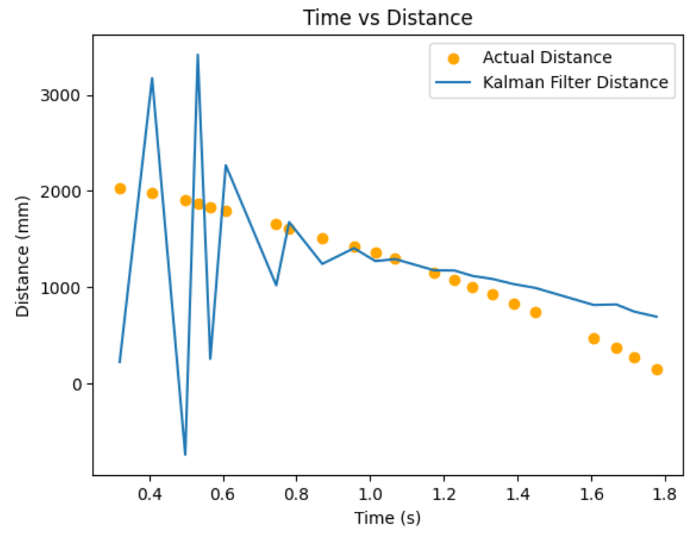
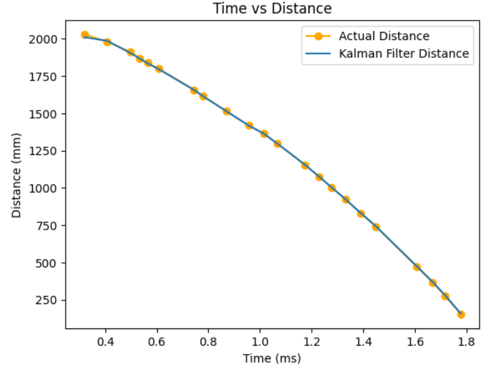
I tested my Kalman Filter with my straight run to the wall data I collected in the beginning of this lab. The orange dots on the graphs below are my ToF sensor data, and my blue line is my estimated Kalman Filter distance. My estimated Kalman Filter distance will help my car estimate when I am exactly 1ft away from the wall quicker. Kalman filter estimated distances complmentry to my slow ToF data will optimze my car's performance.
When I make the uncertainty for my modeled position and my modeled speed low and my uncertainty for my measurement noise high, meaning I put more stress on the model and less on the sensor values, I am very off from the actual data points. Below is my graph when σ1 = 38, σ2 = 38 and σ3 = 108.8.
When I make the uncertainty for my modeled position and my modeled speed really high and my uncertainty for my measurement noise low, meaning I put more stress on the sensor values and less on the model, I get very close to the actual data points. Below is my graph when σ1 = 100, σ2 = 100 and σ3 = 10.
I integrated Kalman Filter into my propotional controller from Lab 6.
I used the drag, mass, dt, and the uncertainty values determined from my simulation when performing Kalman Filter. Whenever I have TOF sensor data, I run the update step of the Kalman Filter, and whenever I don't have TOF sensor data, I run the prediction step. Although, I constantly take data and perform Kalman Filter, I only log every 5 data points due to my ardunio's storage space. Below is my Kalman Filter implementation on Ardunio.
Trial 1:
Trial 2:
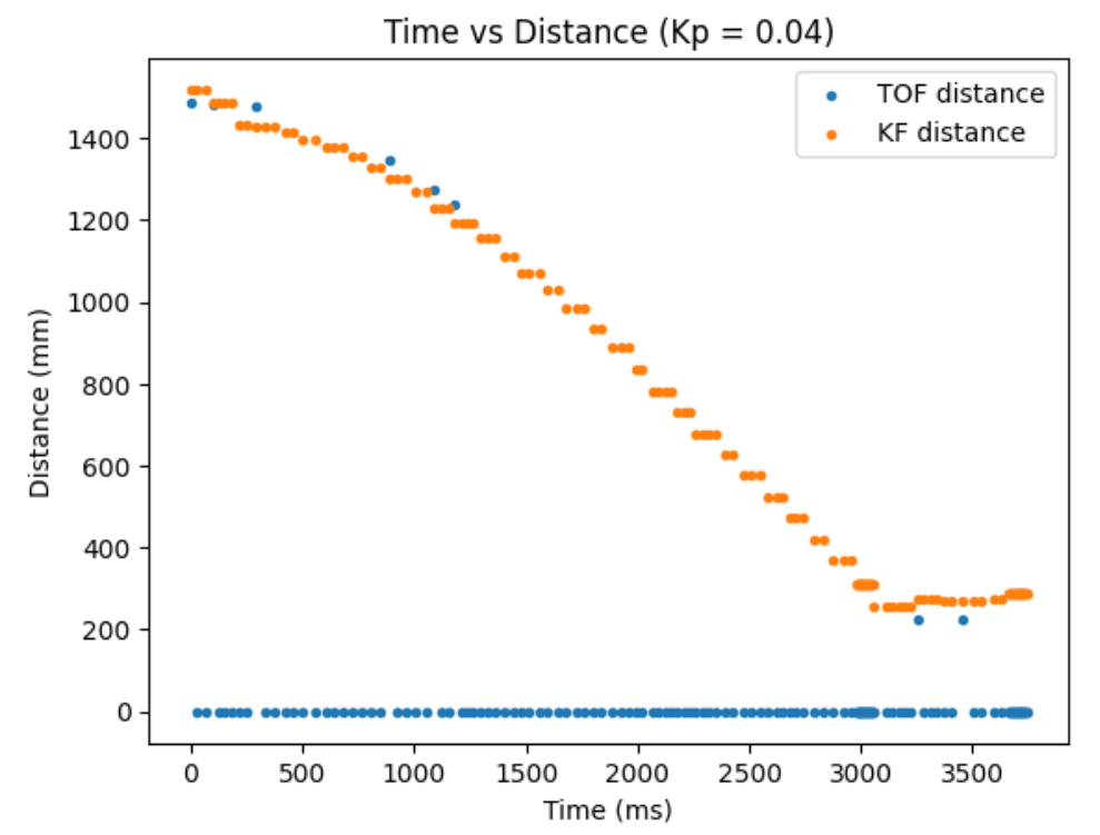
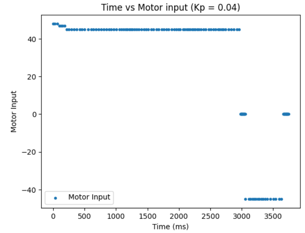
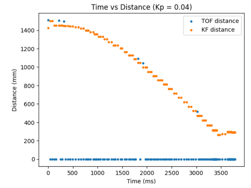
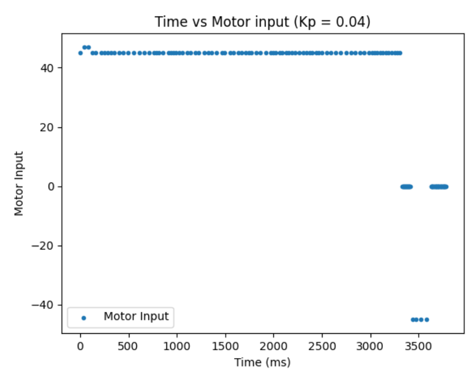
Some reminder from lab 6 is that I limit my motor input between 45 and 255 due to the deadband of the motors. In addition, I found Kp value of 0.04 to work the best for my proportional controller in lab 6, so I used that. A disclaimer is that although the graph shows very few sensor data, this is because I logged every 5 data points and not because my sensor acting weird. When I logged every data, I couldn't log more than 1 second worth of data so, I had to make this exchange.
The graphs from trial 1 and 2 verifies that my Kalman Filter is working correctly. Whenever I don't have sensor data, my robot predicts where I am with the prediction step of the Kalman Filter. As can be seen, the robot has way less oscillation compared to lab 6 and has a quicker settling time when doing a proptional control.
I referenced Anya's lab in performing this lab.
The goal of this lab is for my car to drive forward, do a flip on a sticky matt, and return to where it came from, as fast as possible.
In order to successful perform this lab, I need to do couple of tasks in order:
1. Start at the designated start line
2. Drive forward as fast as possible
3. Upon reaching the sticky matt with a center located 0.5m from the wall, do a flip
4. Drive back in the direction from which it came from, as fast as possible
At first, I tried to do something fancy where I use a combination of PID position control and Kalman Filter to accomplish this task. In order to measure distances upto 360cm away from the wall, I changed the ToF sensors to long distance mode. Distance sensor takes a measurement about every 0.1 seconds. However, since my car is going very fast, at a motor input of 255, the distance sensor's frequency was not fast enough to localize the car at any given time. After numerous unsuccessful tries, I resorted to open loop control--performing each task for a given amount of time range.
After a lot of testing, I concluded on the follow preceedure to accomplish the tasks:
1. Go forward for 1 second while logging distance and speed. This gets me to about the center of the sticky matt. In adddition, this makes sure I have enough momentum to do a flip.
2. Go backward for 0.55 seconds to do a flip. Then stop very briefly, for 0.04seconds, to make my motors not spin while I am flipping. When I don't stop turning my wheels while I am flipping, I realized the momentum of the wheel spinning causes my car to jerk or make one of the spinning wheels touch the ground first, causing my car to be off angled.
3. Go backward for 0.95 seconds to come back to the start line.
Battery level affected how fast or slow my car moved, but the preceedure above proved to be quite reliable. On average, I do the entire stunt in about 2.8 seconds. My fastest run was about 2.5 seconds.
Below is my stunt code in Ardunio:
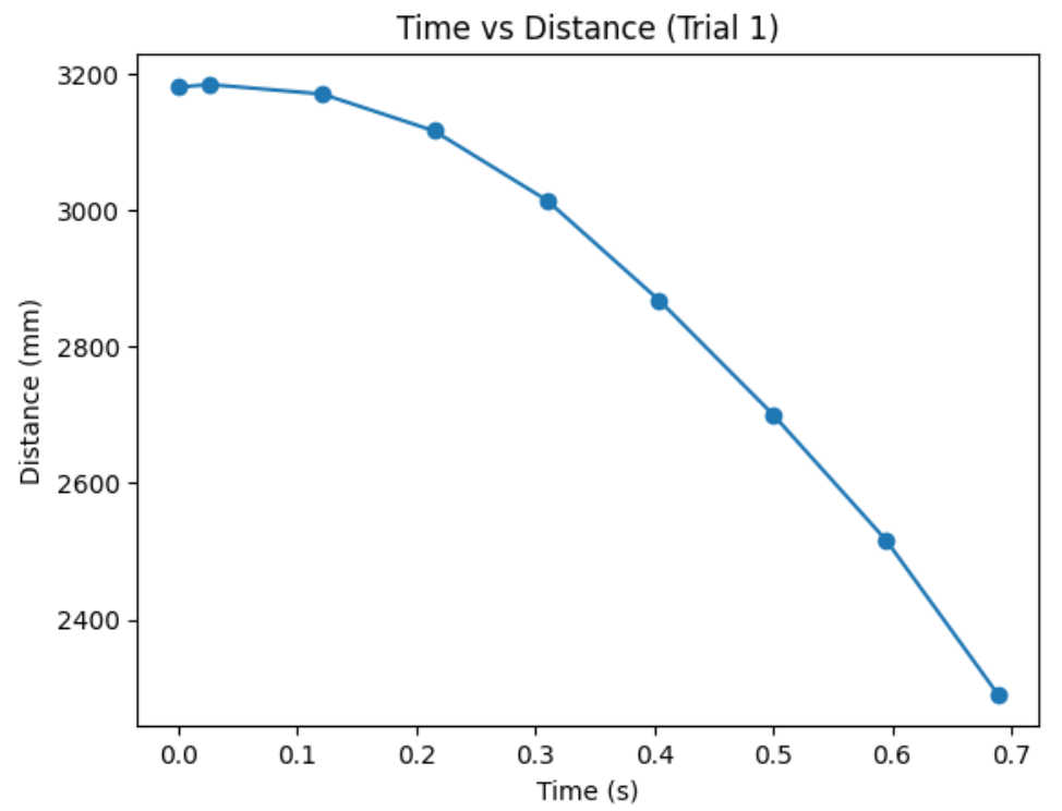
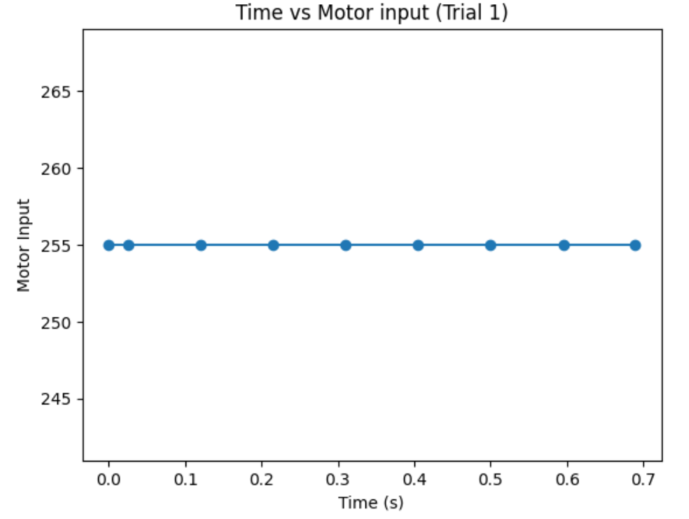
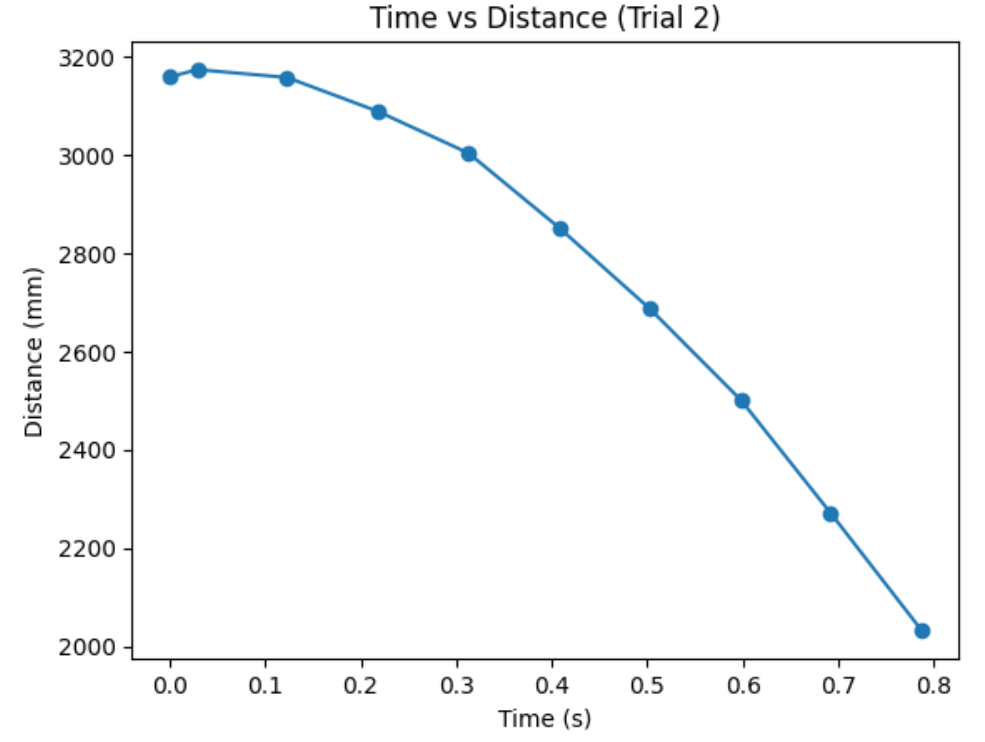
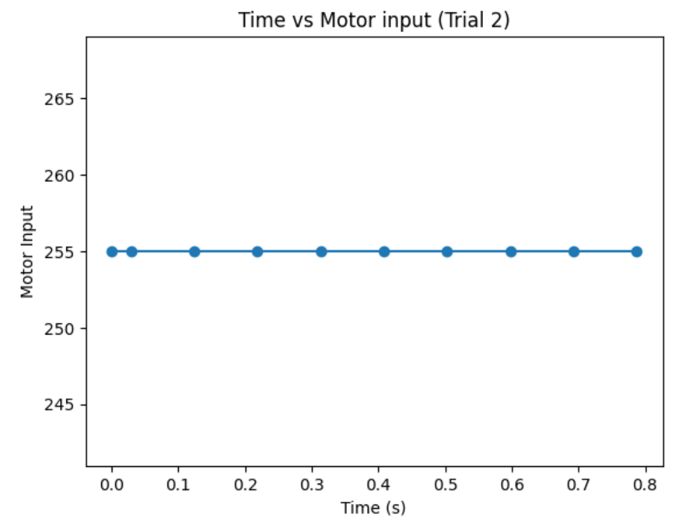
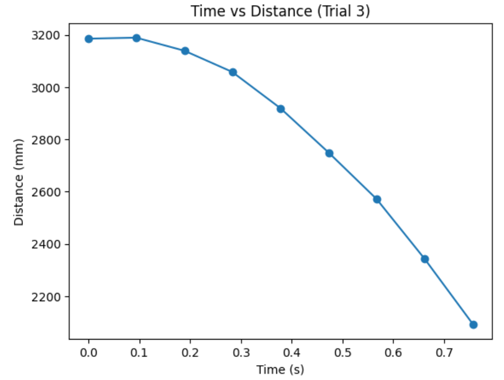
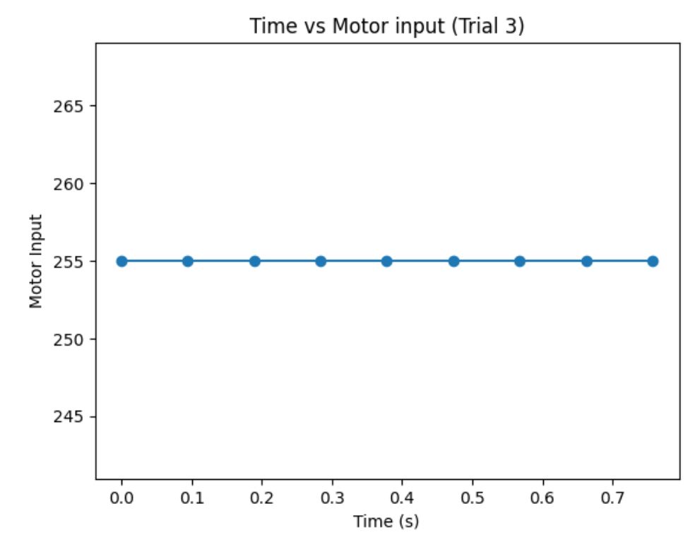
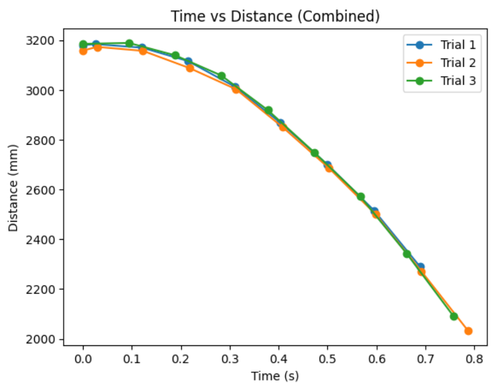
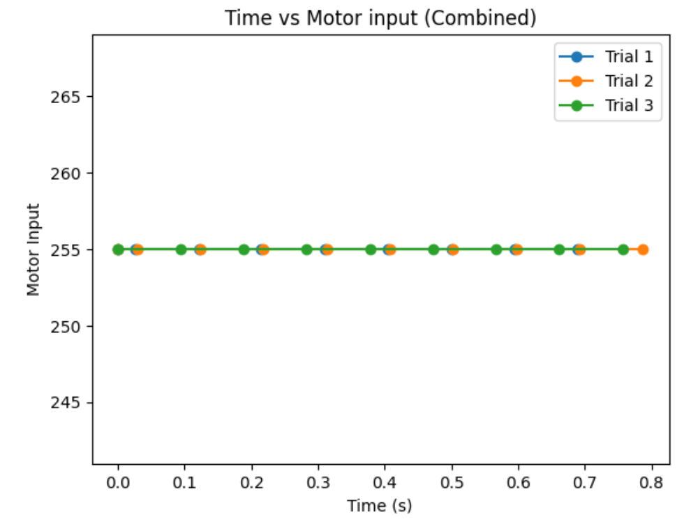
The combined graph shows how the task is repeatable. In addition, it shows that distance sensor's frequency is not fast enough to localize the car at any given time. The last distance measurement, before the flip, is at about 200cm. However, the robot is actually at around 50cm from the wall.
Here are all the blooper vidoes from testing. Enjoy!
The goal of this lab is to map out a static room by placing the robot at couple different locations of the room and merging the results.
In order to create a good quailty map, I decided to do angular speed control. I created a proportional controller that works directly on the raw angular velocity of my robot turning. This is beneficial over orientation control because I can avoid gyroscope drift, which is accumulating errors during integration.
From lots of testing, I found out that my robots spins better when I turn right (CW) compared to when I turn left (CCW). In addition, my robot turns most axially and steady with the motor input value of 110 (with the deadband below 70), an angular speed of 70, and Kp of 1. Below is my code snippet to do proportional control on angular speed.
Below is my robot spinning, roughly on axis, with the proportional controller. The wheels are tapped in order to minimize friction when rotating.
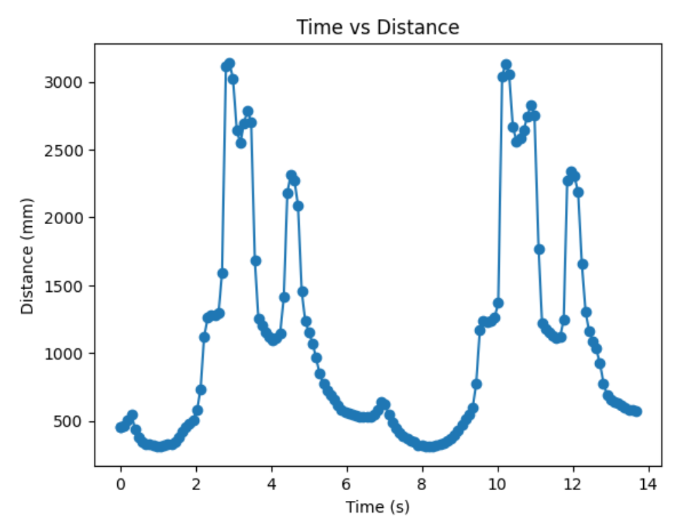
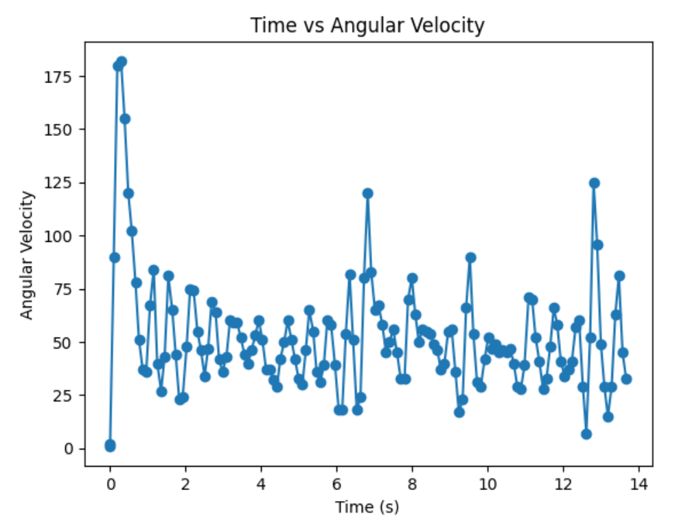
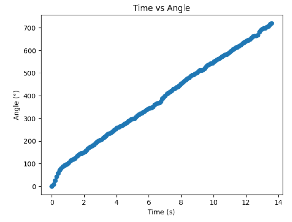
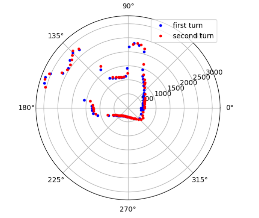
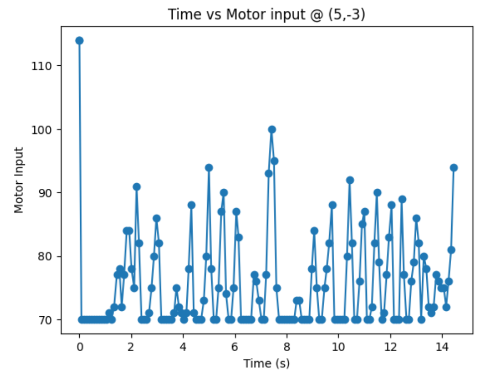
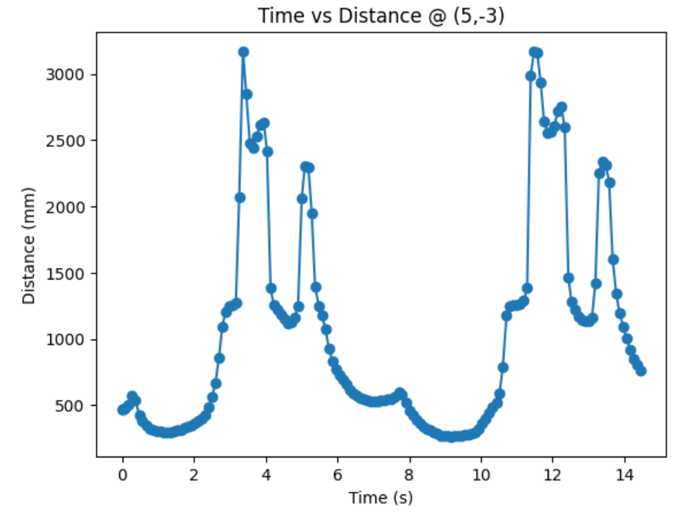
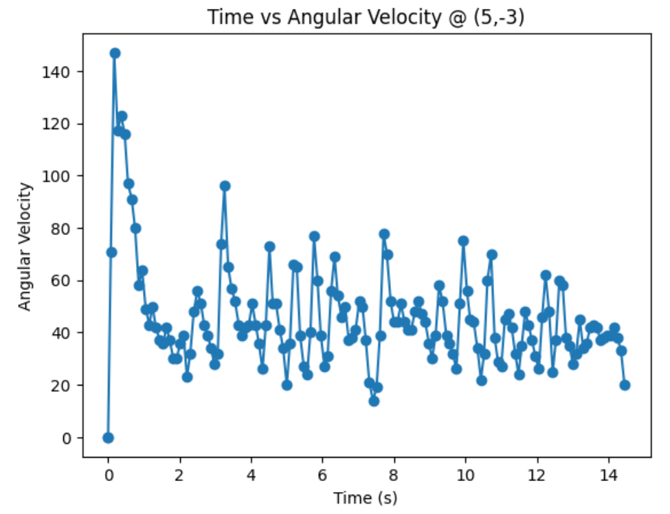
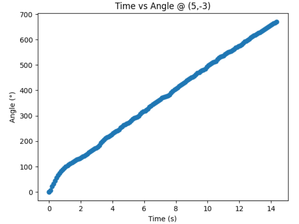
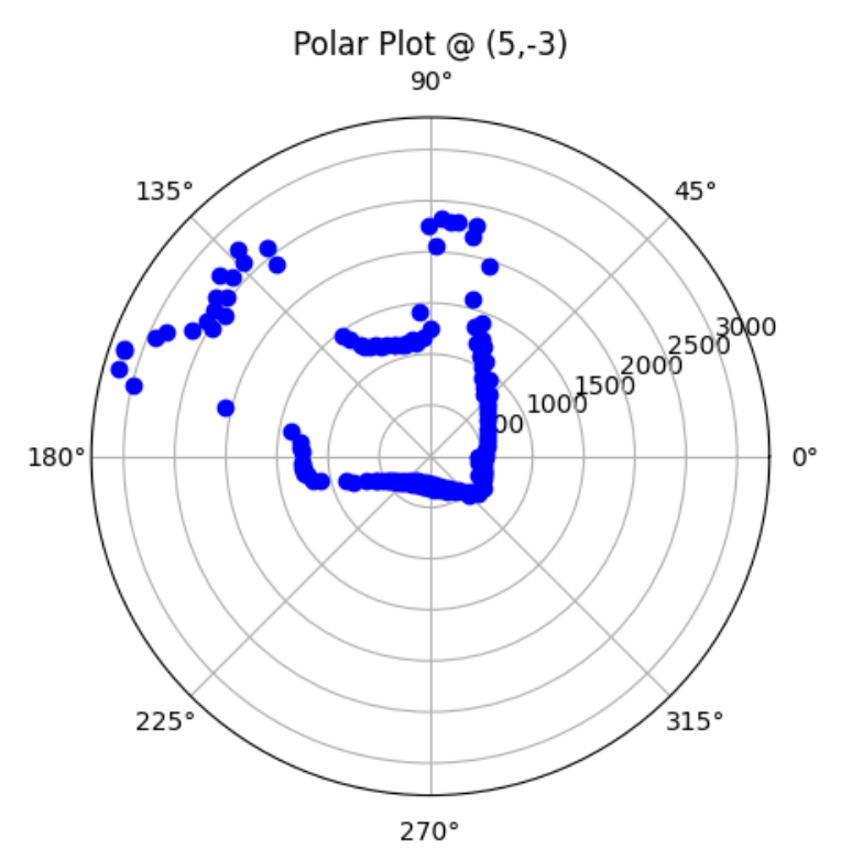
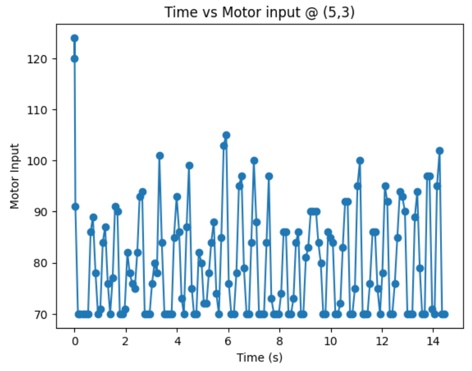
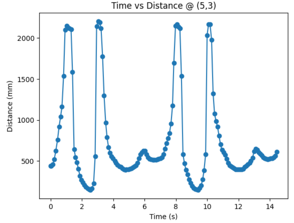
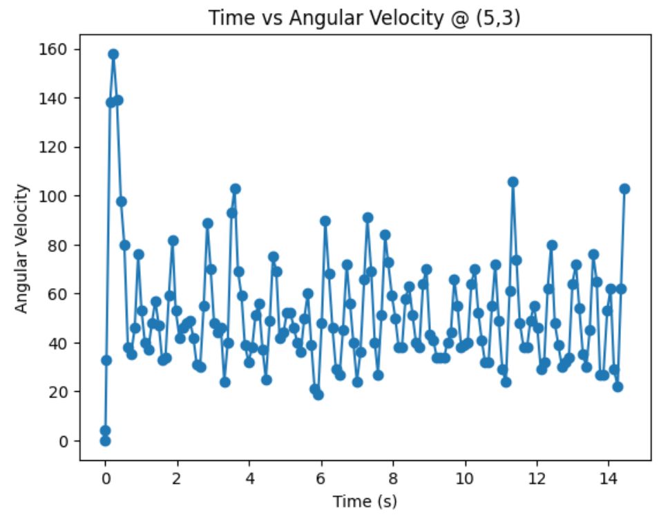
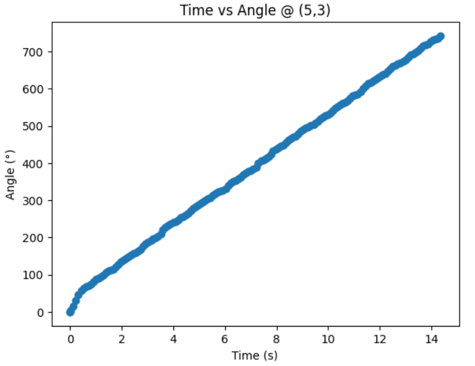
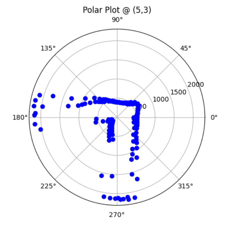
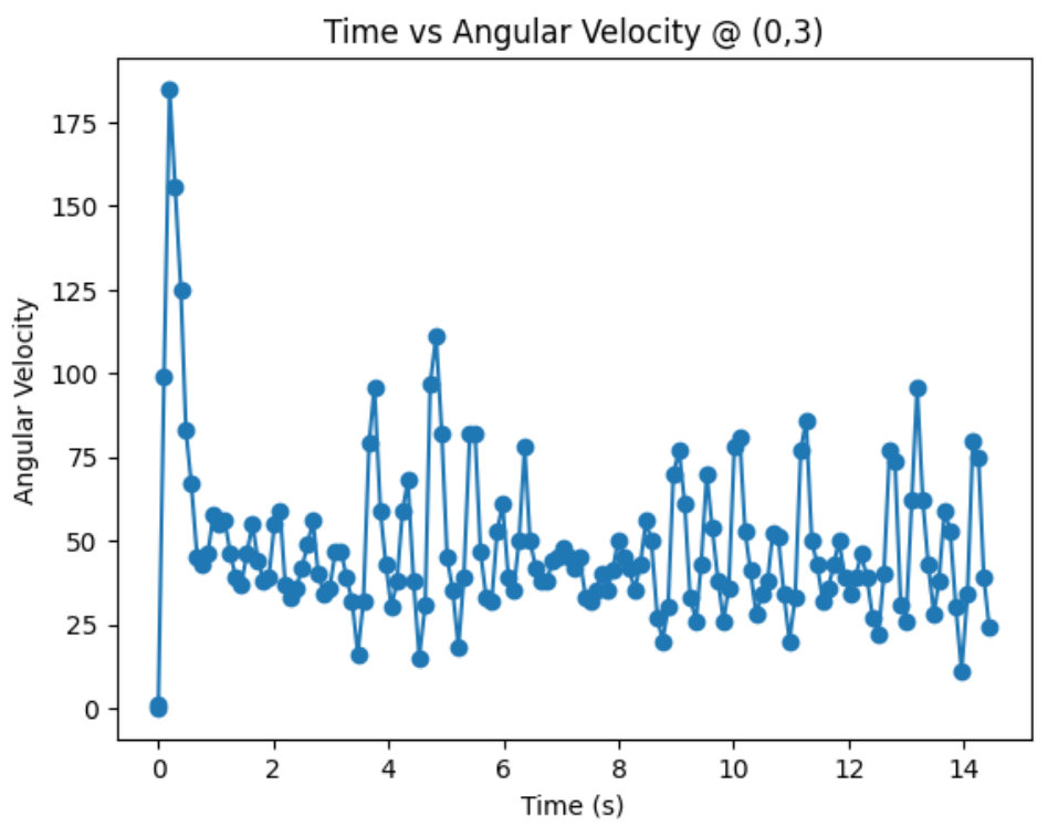
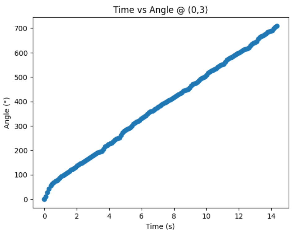
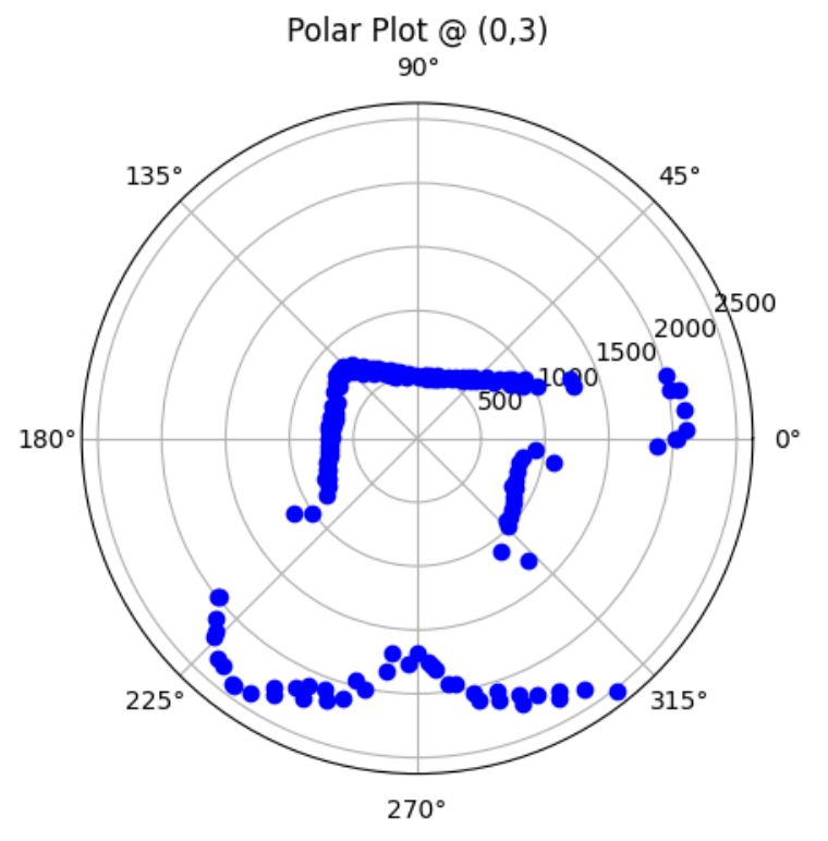
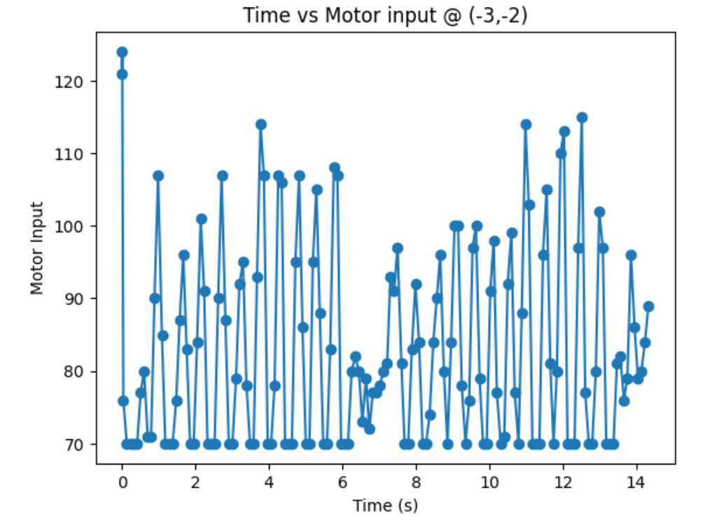
Graphs below show my data readings when my robot turns two full rotations. I collected 144 data points during the two rotations. That is about 72 data points per 360 degrees, which is equivalent to a data point per 5 degrees in rotation. My time vs distance graph looks pretty similar in the first and second rotation. It can be observed at my angular speed tries to remain relatively constant, due to the proportional controller. The time vs angle graph looks like it is steadly increasing. These findings can be verified in the polar graph. The map from the first rotation and the second rotation seems very close to each other.
Below is my robot spinning with open loop control. Theortically, my robot is supposed to give more uniformly spaced out and more on axis spin data with angular speed control. However, the bad quailty of my motors made my open loops control spin better than angular speed control. Although my open loop control performs better, in order to get fully credit on this lab, I will use angular speed control.
I placed my robot in four of the marked positions in the lab space and recorded data for two full rotations. Below are the results.
Bottom Right Corner (5,-3):
Top Right Corner (5,3):
Top Middle Corner (0,3):
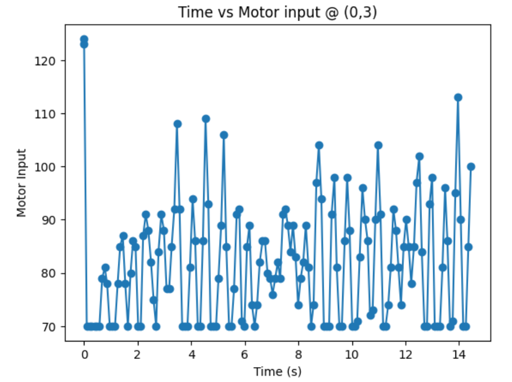
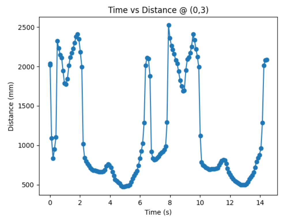
Bottom Left Corner (-3,-2):
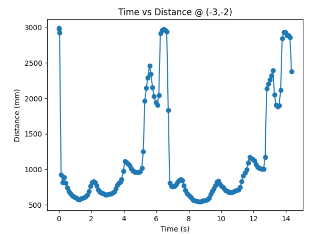
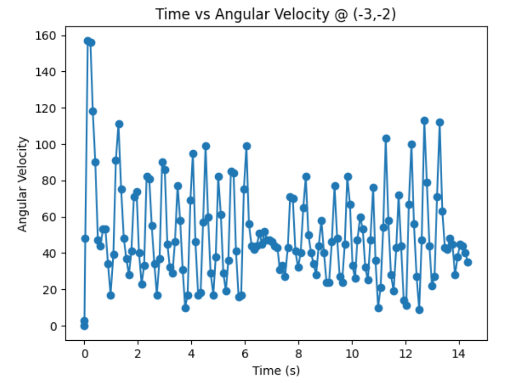
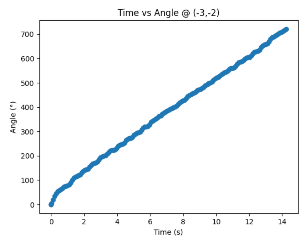
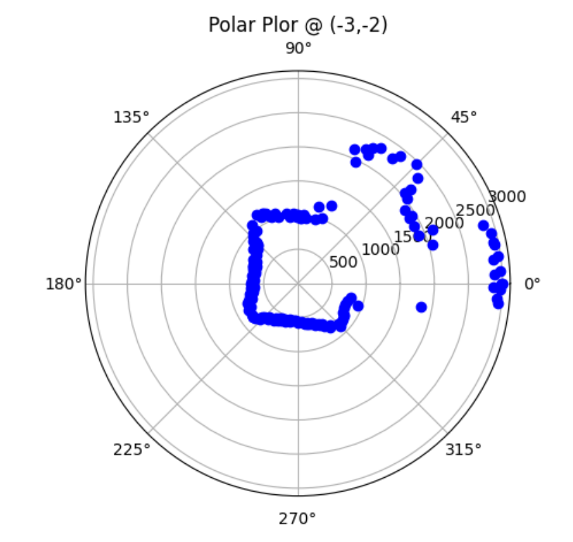
I need to convert measurements from the distance sensor to the inertial reference frame of the room. I will do that by doing x = dist*cos(angle) + inital_x_pos and y = dist*sin(angle) + inital_y_pos. Since distance sensor readings are in mm and my inital positions are in feet, I will convert feet to mm.
#bottom right = (5,-3)
x_br = d_br*np.cos(ar_br) + (5*304.8)
y_br = d_br*np.sin(ar_br) - (3*304.8)
#top right = (5,3)
x_tr = d_tr*np.cos(ar_tr) + (5*304.8)
y_tr = d_tr*np.sin(ar_tr) + (3*304.8)
#top middle = (0,3)
x_tm = d_tm*np.cos(ar_tm)
y_tm = d_tm*np.sin(ar_tm) + (3*304.8)
#bottom left = (-3,-2)
x_bl = d_bl*np.cos(ar_bl) - (3*304.8)
y_bl = d_bl*np.sin(ar_bl) - (2*304.8)


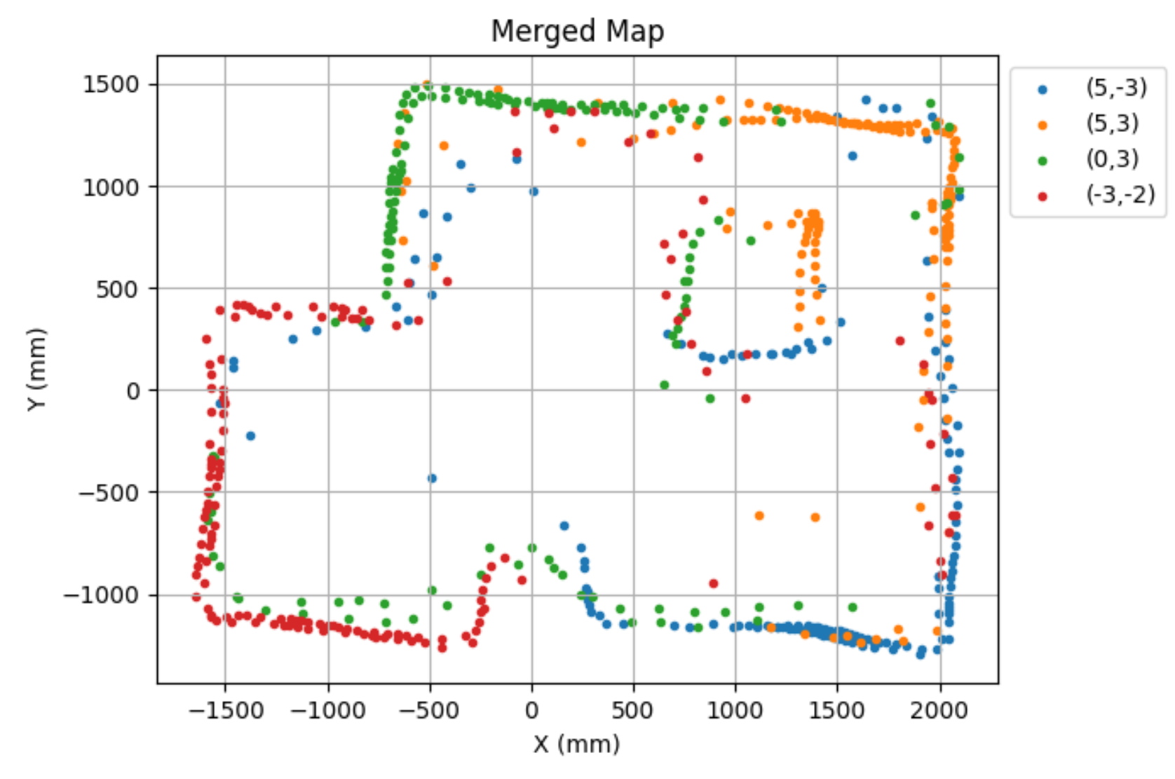
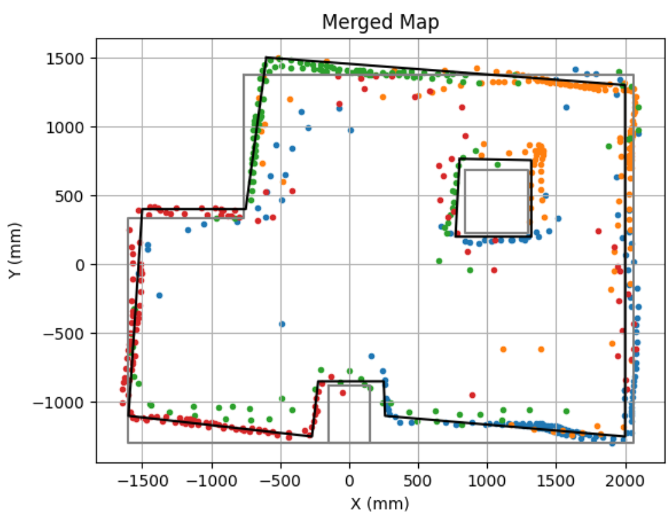
I want to convert this map into a format I can use later in the later labs. So, I will manually estimate where the actual walls and obsticles are based on my scatter plot.
#estimated walls/obsticles
wall_x = [-600, 2000, 2000, 260, 250, -225, -270, -1600, -1500, -750, -600]
wall_y = [1500, 1300, -1250, -1100, -850, -850, -1250, -1100, 400, 400, 1500]
obsticle_x = [800, 1320, 1320, 770, 800]
obsticle_y = [765, 755, 200, 200, 750]
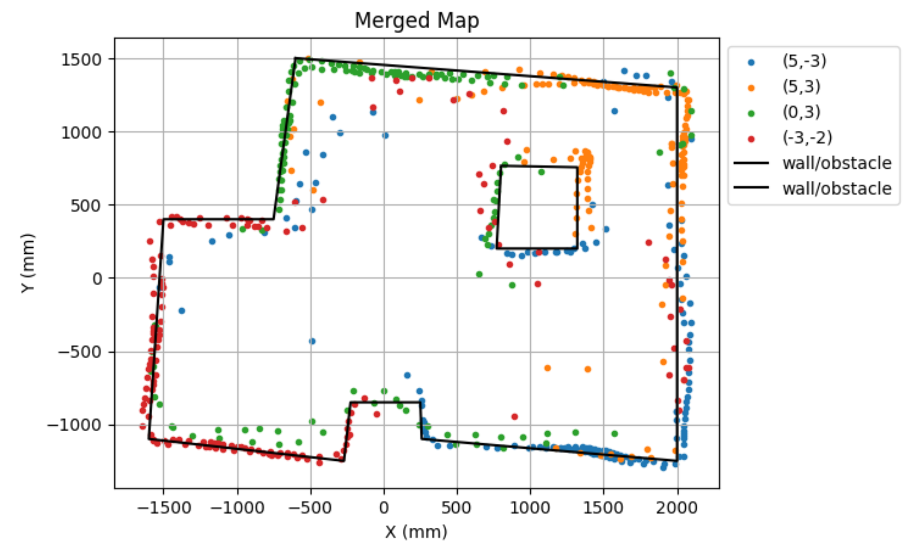
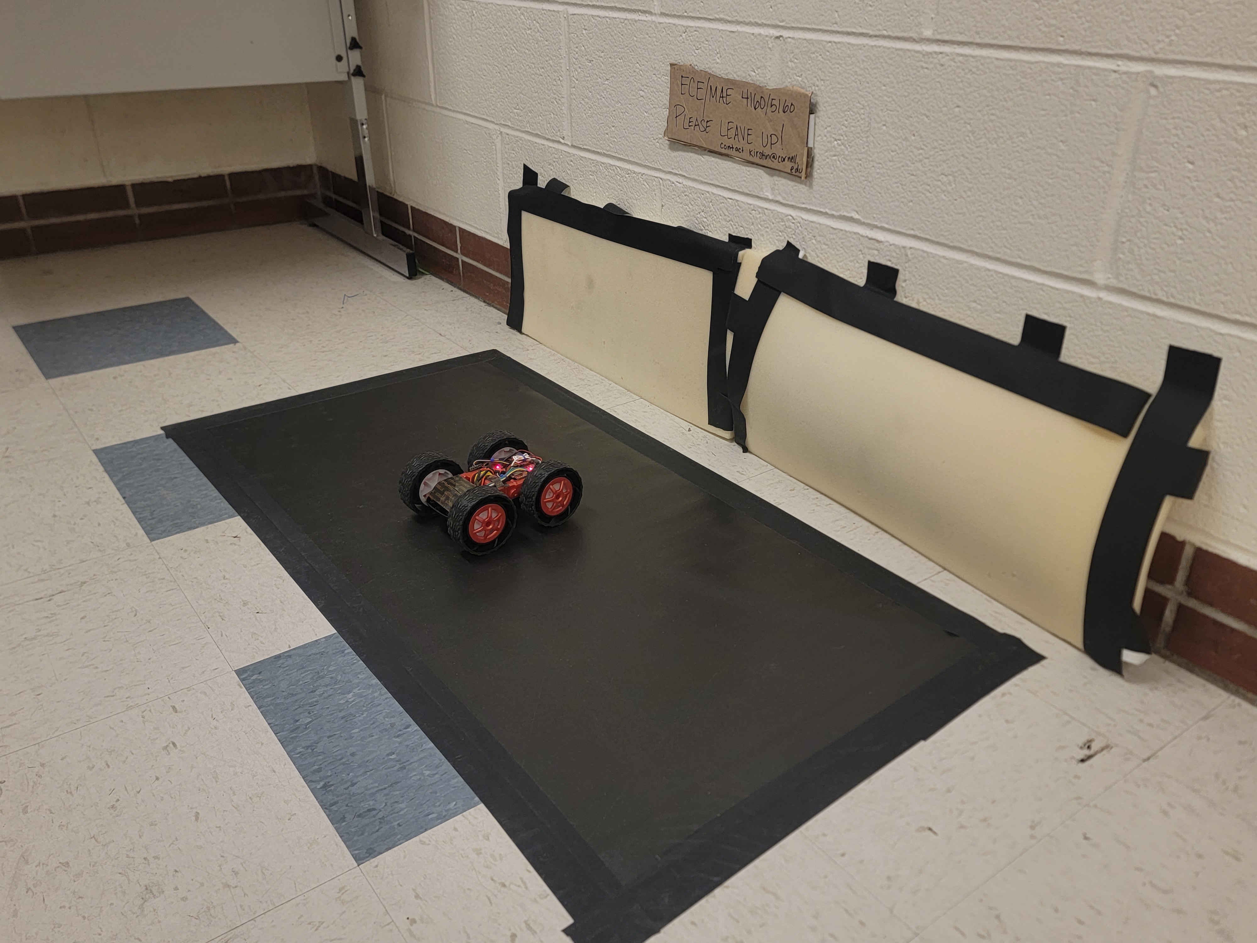
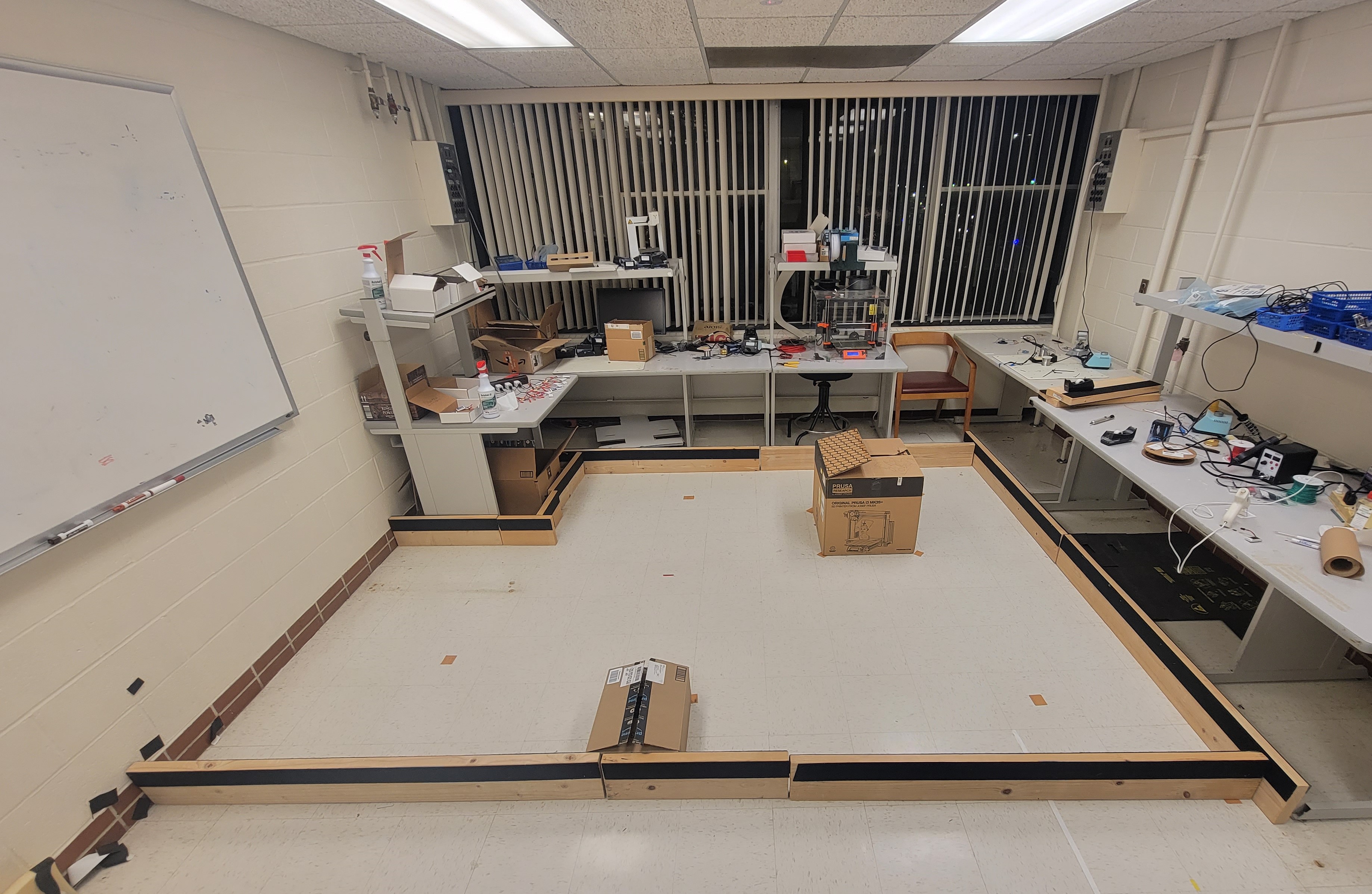
This is the actual set up of the map. As can be seen, some walls of the actual set up were crooked. This probably the cause of my merged map looking croocket on some sides. In the future labs, I will make sure the set up is not crooked before performing the lab tasks.
Theoretically, if my set up wasn't croocked, I think my walls and obsticles would have been closer to the list below.
#theoretical walls/obsticles
wall_x = [ -762, 2057.4, 2057.4, -1600.2, -1600.2, -762, -762]
wall_y = [ 1371.6, 1371.6, -1295.4, -1295.4, 335.28, 335.28, 1371.6]
box1_x = [-152.4, 152.4, 152.4, -152.4, -152.4]
box1_y = [ -883.92, -883.92, -1295.4, -1295.4, -883.92]
box2_x = [ 838.2, 1295.4, 1295.4, 838.2, 838.2]
box2_y = [685.8, 685.8, 228.6, 228.6, 685.8]
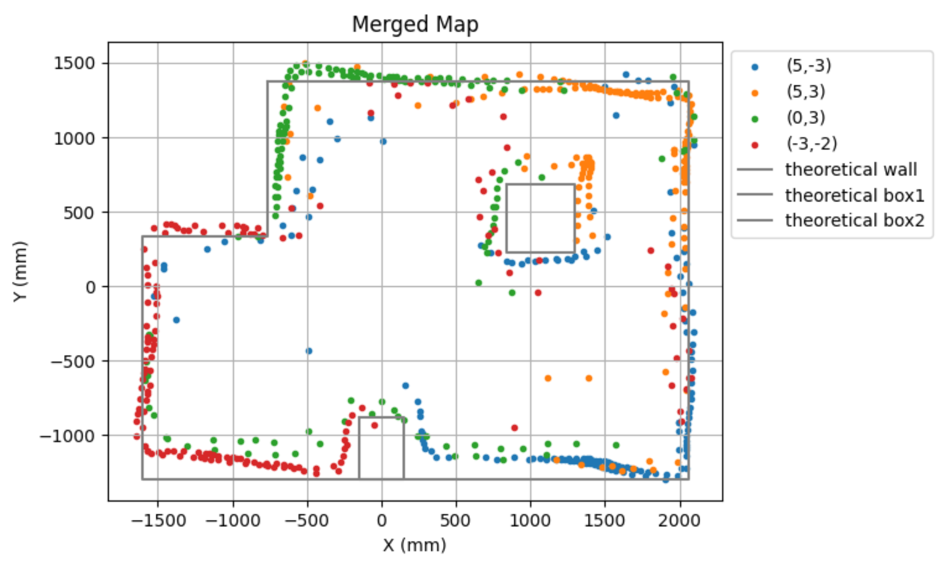
Lastly, this is my line based map with my estimated and theortical walls and obsticles.
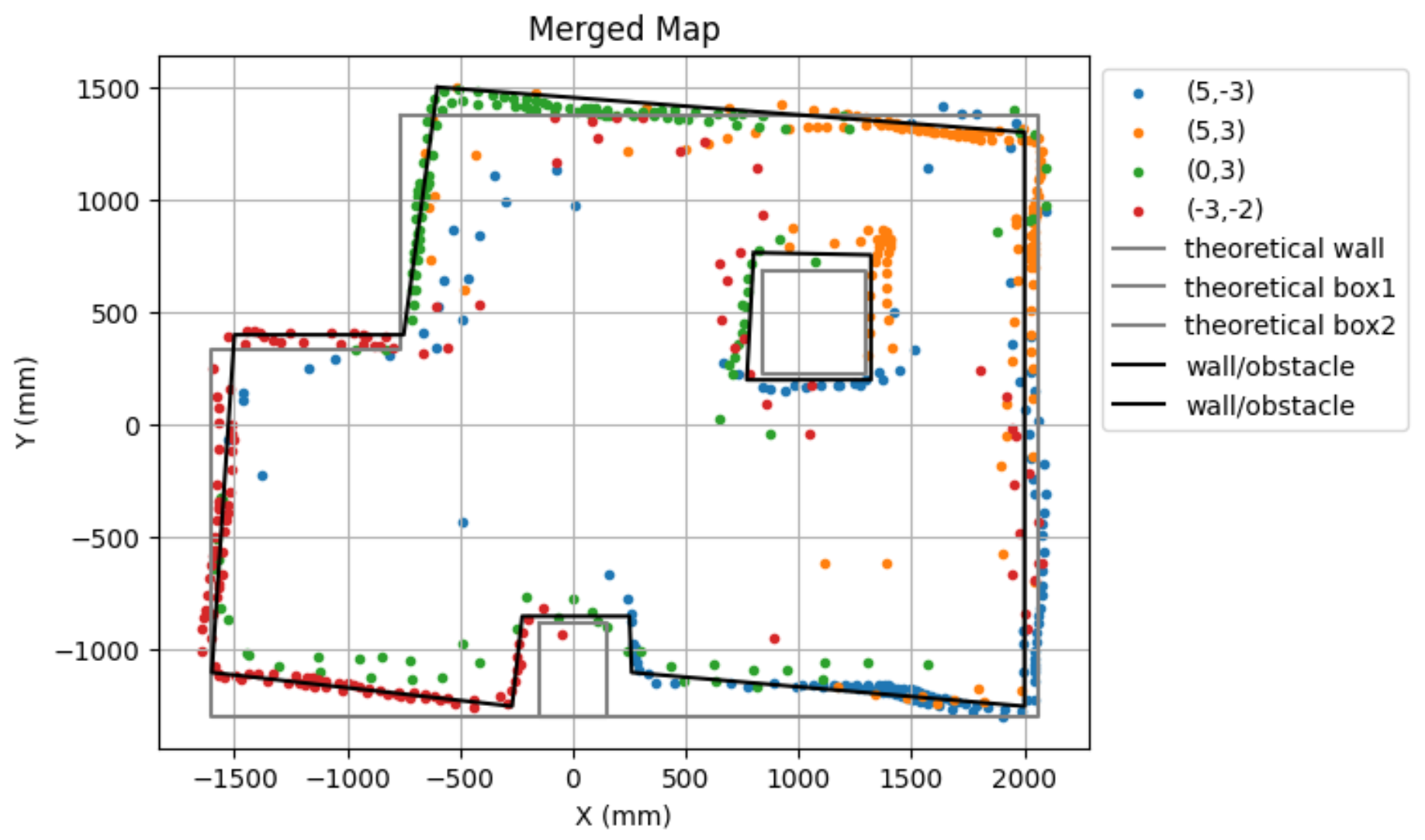
I referenced Anya's lab in performing this lab.
The goal of this lab is to do grid localization with Bayes Filter in the simulation.
In this lab, I want to perform grid localization for the smaple trajectory. I started by downloading the lab10 notebook from here.
Our state space is modeled as a finite 3D grid space, compoased of x, y, and θ. This means we won't be able to distinguish the robot's state if it is in the same grid cell, but this is good enough for our purposes and for computation time. Resolution of the x, y, and θ cell is 0.3048m, 0.3048m, and 20 degrees, and the number of cells are 12 by 9 by 18. Each grid cell is composed of the probabilty of the robot's presence in that cell. This probability is updated through the Bayes filter. Measurement noise and control data noise is modeled by Gaussian Distribution.
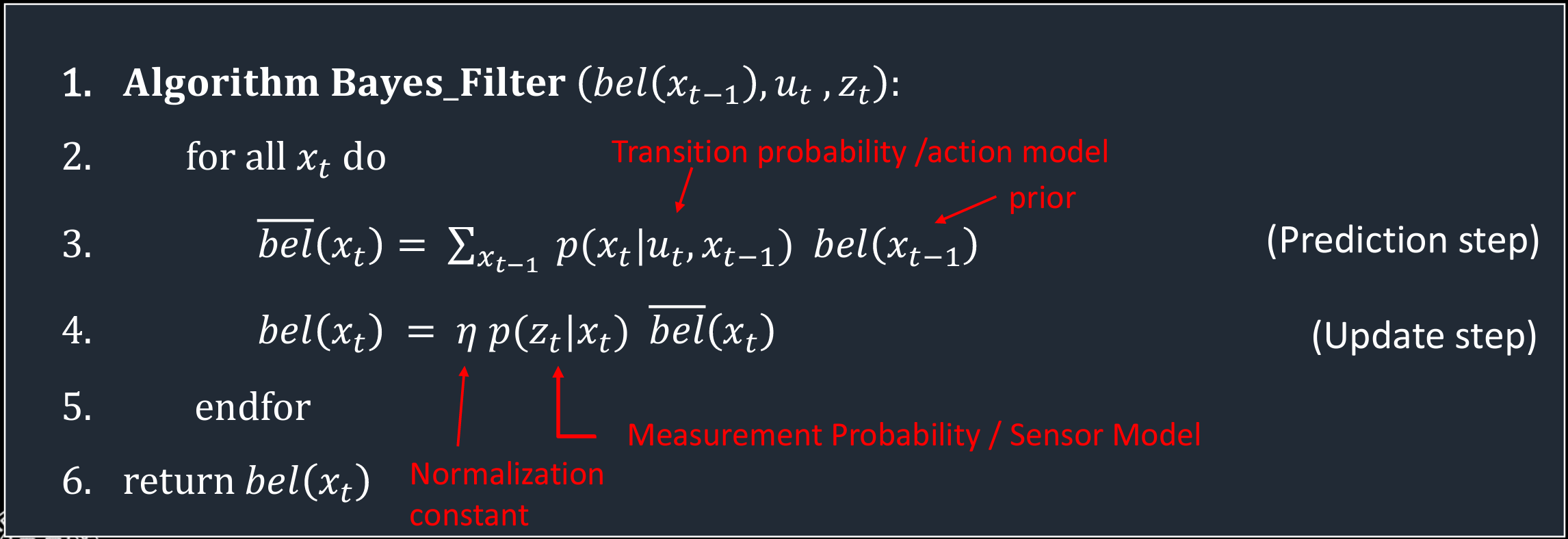
As shown below, Bayes filter has two main steps every iteration: prediction and update. Prediction step uses the control input data from movement. Prediction step increases belief uncertainty. Update step uses the obervation data from measurement. Update step reduces uncertainty.
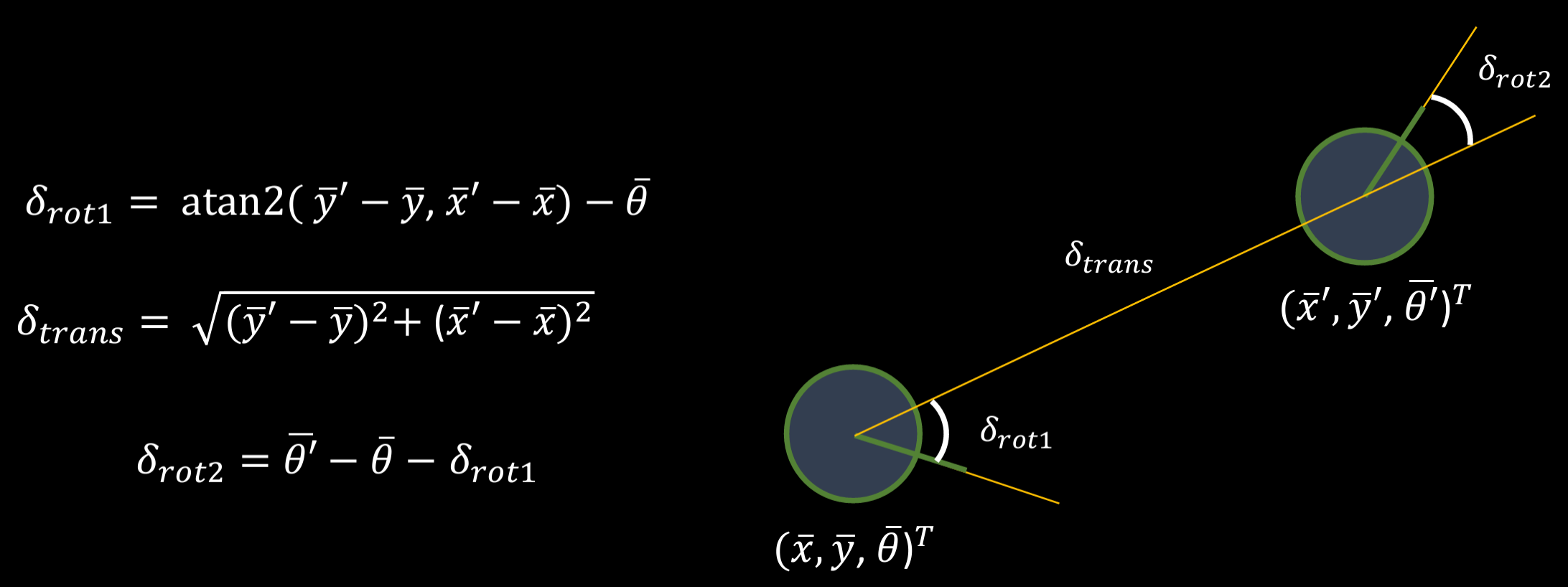
This function takes in the current and previous pose and returns rotation 1, tranlation, and rotation 2. Each pose is composed of x, y, and orientation (yaw). The image below shows a good visual representation of the poses' relation.
Below is my code snippet to do to compute_control.
This function takes in current pose, previous pose, and u and returns the probability. This is done by plugging in actual u and u into a gaussian function to see how "probable" is the transition from the previous pose to the current pose, given the actual control action. The image below shows the formula to calculate this probability.

Below is my code snippet to do to odom_motion_model.
This function takes in current pose and previous pose and updates the probabilites in the loc.bel_bar. The image below shows the mathmatical formula for the prediction step. I was able to accomplish this with the use of 6 forloops

Below is my code snippet to do to prediction_step.
This function takes in a 1D array of true observations for a specific pose in the map and returns a 1D awway of size 18 with the likelihoods of each sensor measurement. The image below shows a mathmatical formula to find the likelihood of the 18 true measurements given the state.

Below is my code snippet to do to sensor_model.
This function updates the probabilities in loc.bel based on loc.bel_bar and the sensor model. The image below shows the mathmatical formula for the update step of the Bayes Filter.

Below is my code snippet to do to undate_step.
Below is a video of my Bayes Filter working on a preplanned trajectory. The left graph is the trajectory plotter and the right graph is flatland.
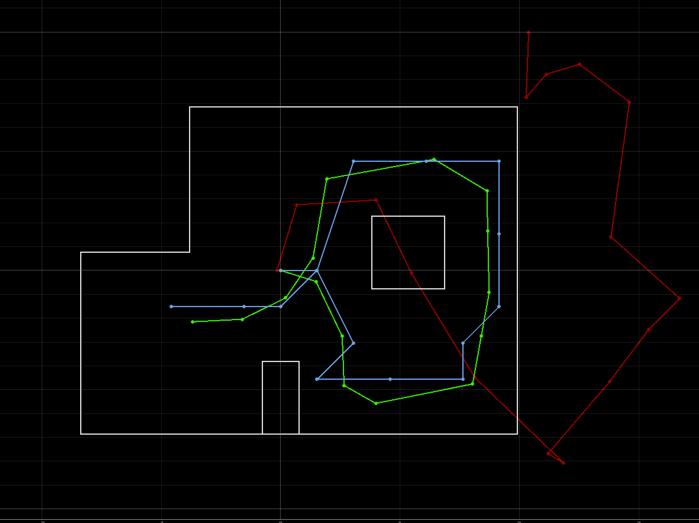
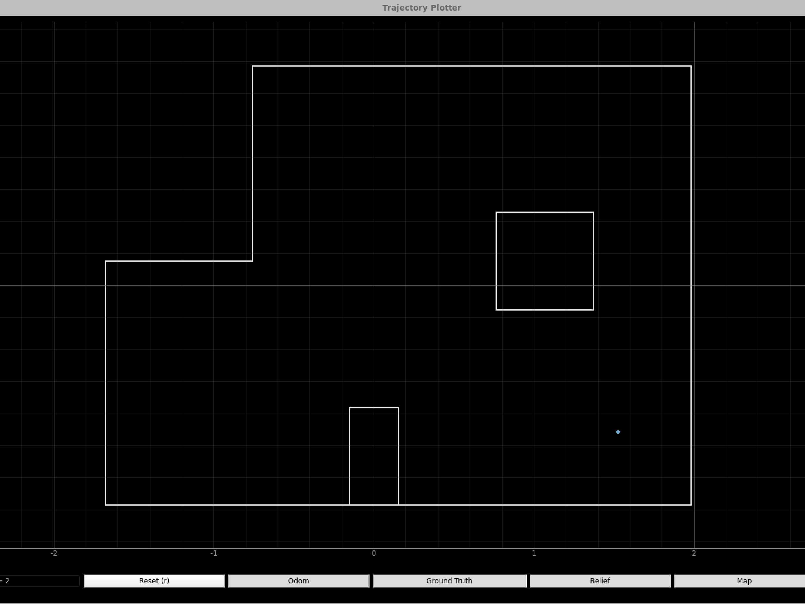
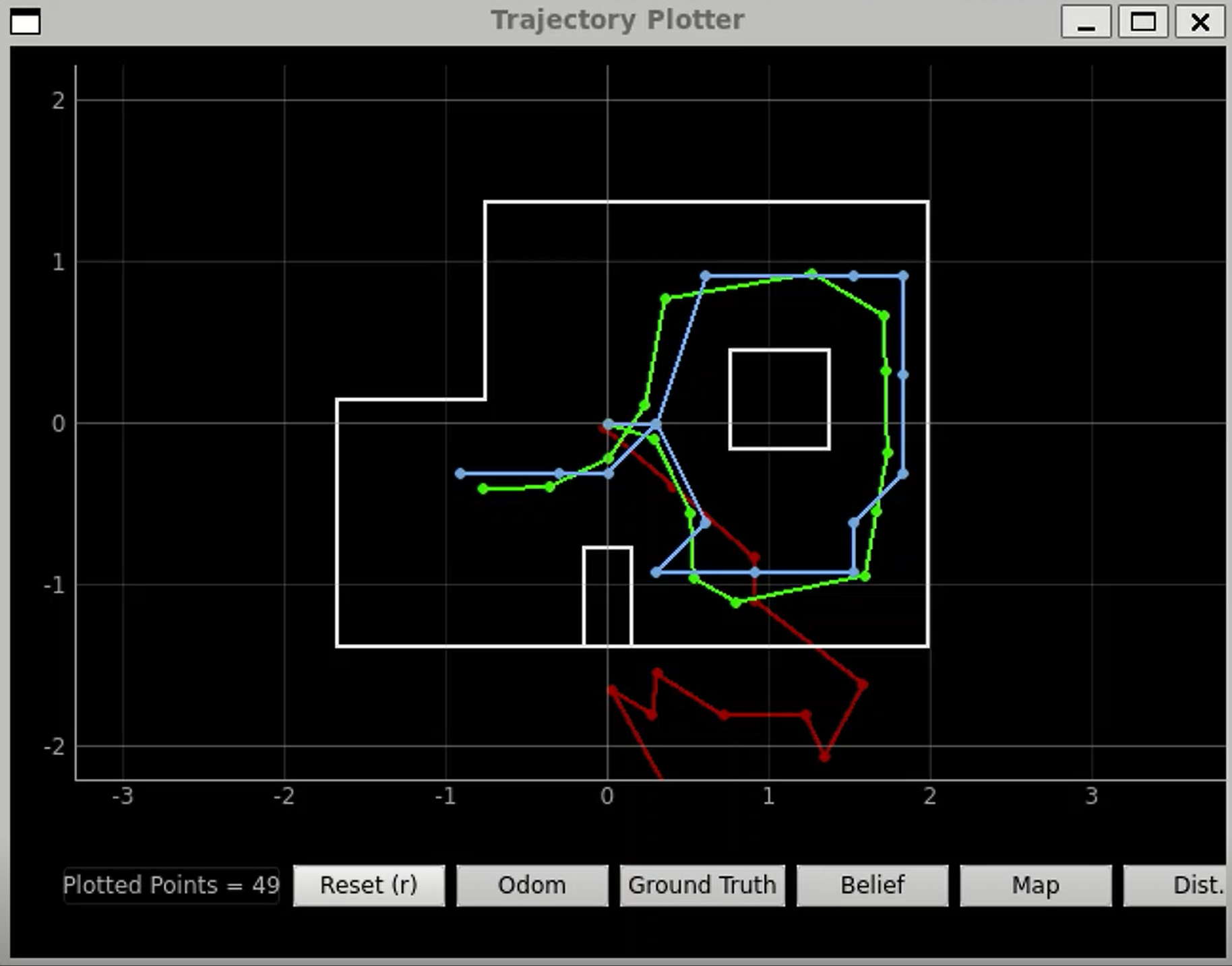
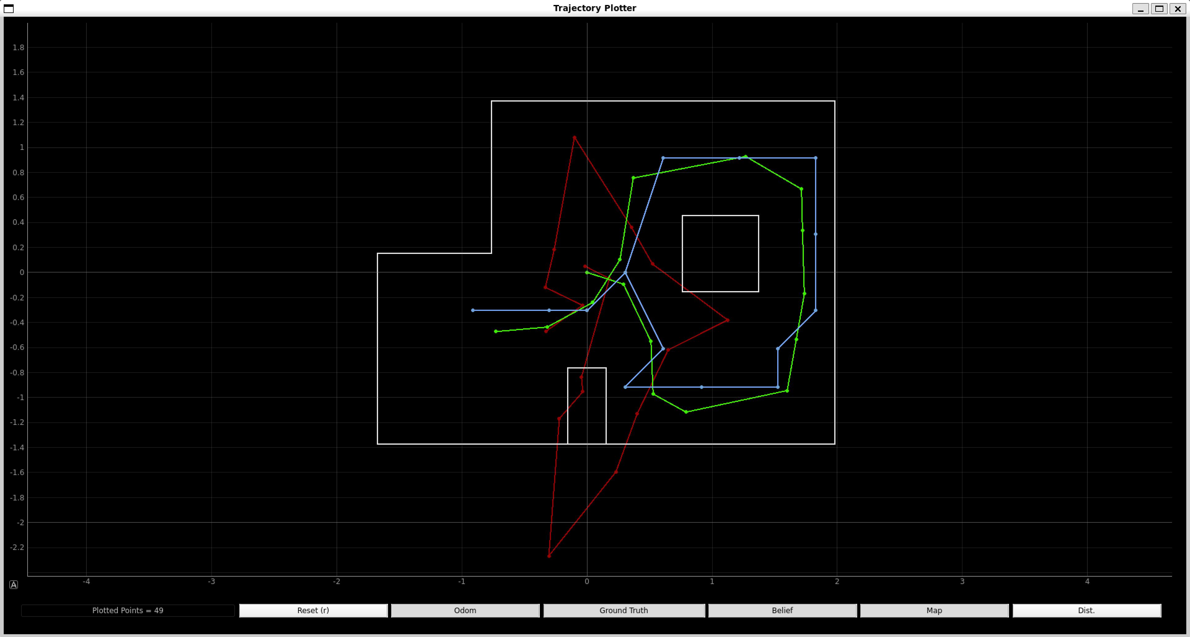
Below is the graph from the trajectory plotter. The white lines represent the map. The red path is the odometry, the green path is the ground truth, and the blue path is the belief. My ground truth path and the belief path are near each other, signifying that my Bayes Filter worked.
Below is the logged update stat and the prediction stat, printed in Jupyter Notebook.
I referenced Anya's lab in performing this lab.
The goal of this lab is to do grid localization with Bayes Filter on the real robot.
I collaborated with TianTian Li on this Lab!
We ran our provided notebook lab11_sim.ipynb, which is an optimized Bayes filter implementation that works on the virtual robot. Below is the final plot of the trajectory plotter. The red path is the odometry, the green path is the ground truth, and the blue path is the belief. It can be verified that the simulator gives similar results to Lab 10.
We went through the lab11_real.ipynb and implemented the perform_observation_loop(self, rot_vel=120) function. Rest of the given code makes it possible for us to run the update step using the sensor measuement data to localize our real robot. The given code used only the update step from a one full rotation since the rotation of the robot is so noisey that the prediction step doesn't really help.
We used the asyncio.sleep() function for the first time in writing the perform_observation_loop(self, rot_vel=120) function. We did this by adding the keyword async to the function definition, placing the keyword await infrot of asyncio.sleep(), placing the await keyword whenever calling the async coroutine perform_observation_loop(), and by placing the await keyword to the line loc.get_observation_data(). Below is our code snippet of our implementation of the perform_observation_loop(self, rot_vel=120) on Jupyter.
Below is our code snippet to do localization on the ardunio. The code is essentiially the same my my mapping_pid() function from my lab 9 except that this time around, I make my robot do a one full rotation instead of two full rotations.
Now that all the code is implemented, we placed out robot in the four marked poses and ran the updated step of the Bayes filter. The blue dot is the belief, and the green dot is the ground truth.
Bottom Right Corner (5, -3, 0 deg):


Top Right Corner (5, 3, 0 deg):
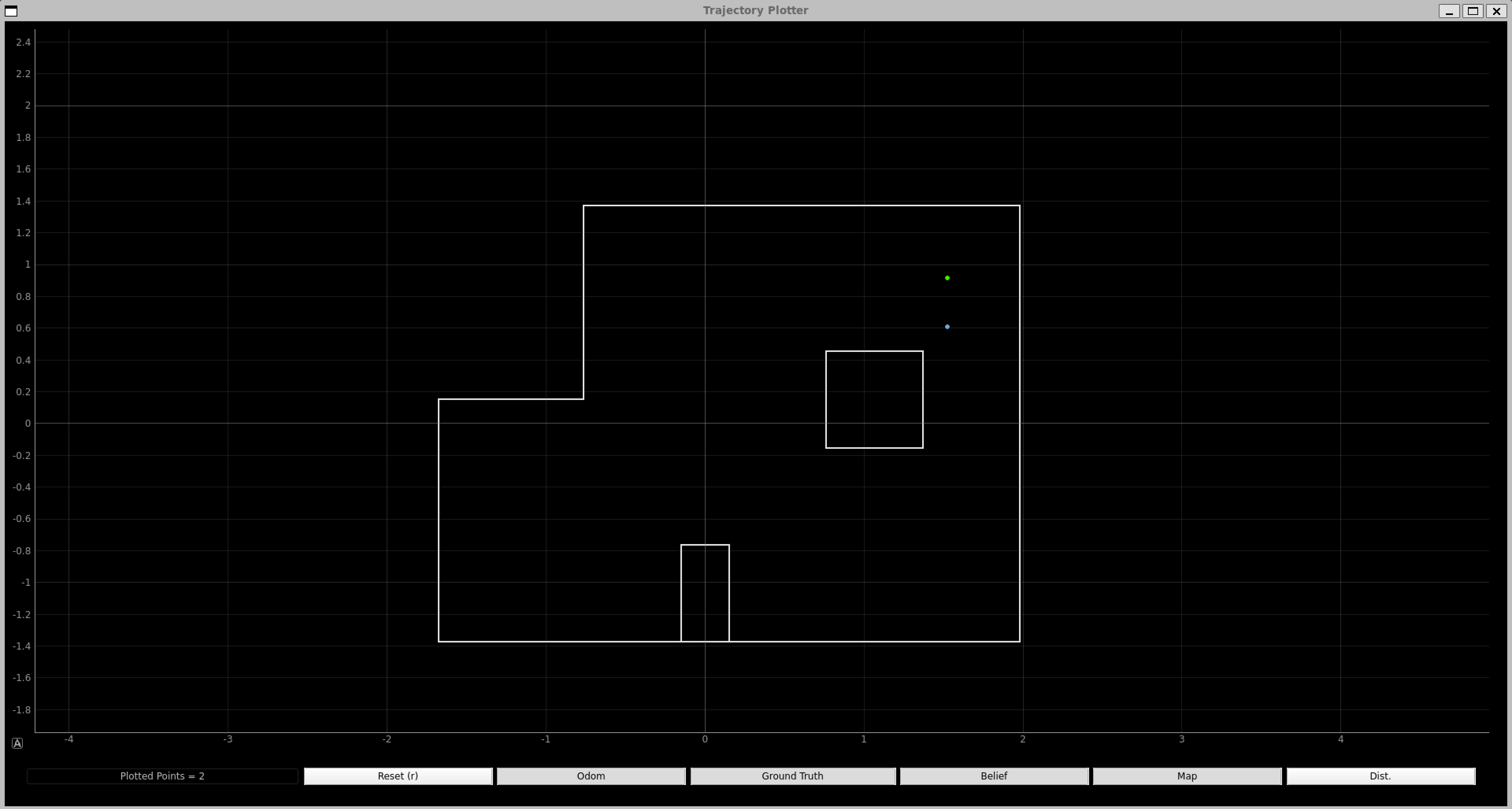

Top Middle Corner (0, 3, 0 deg):
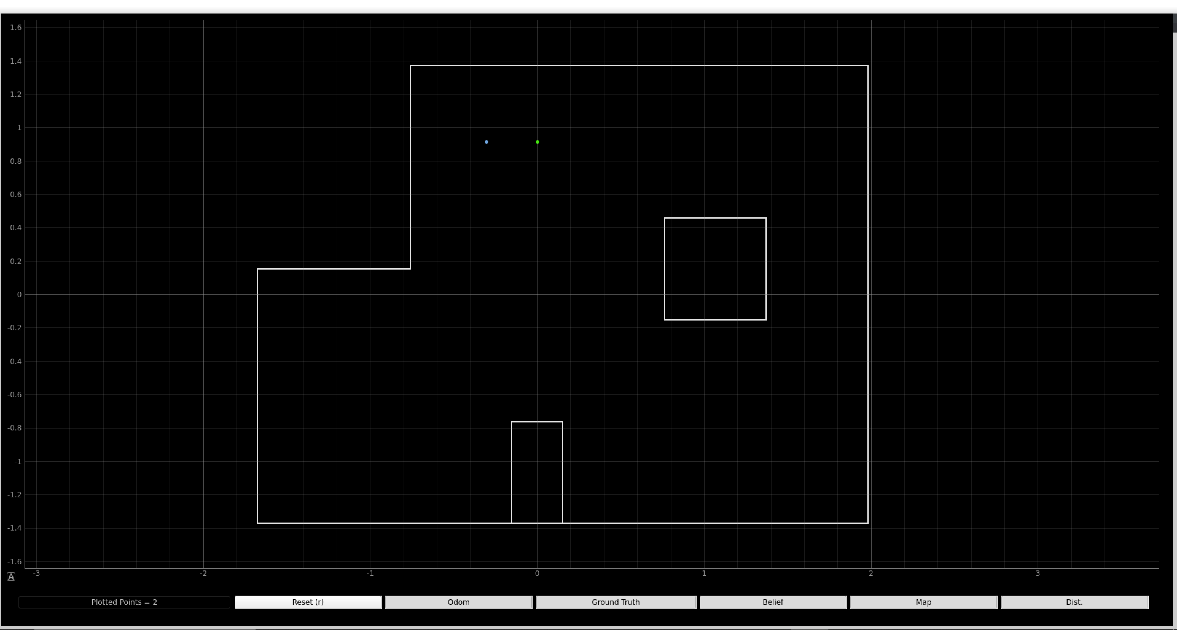

Bottom Left Corner (-3, -2, 0 deg):
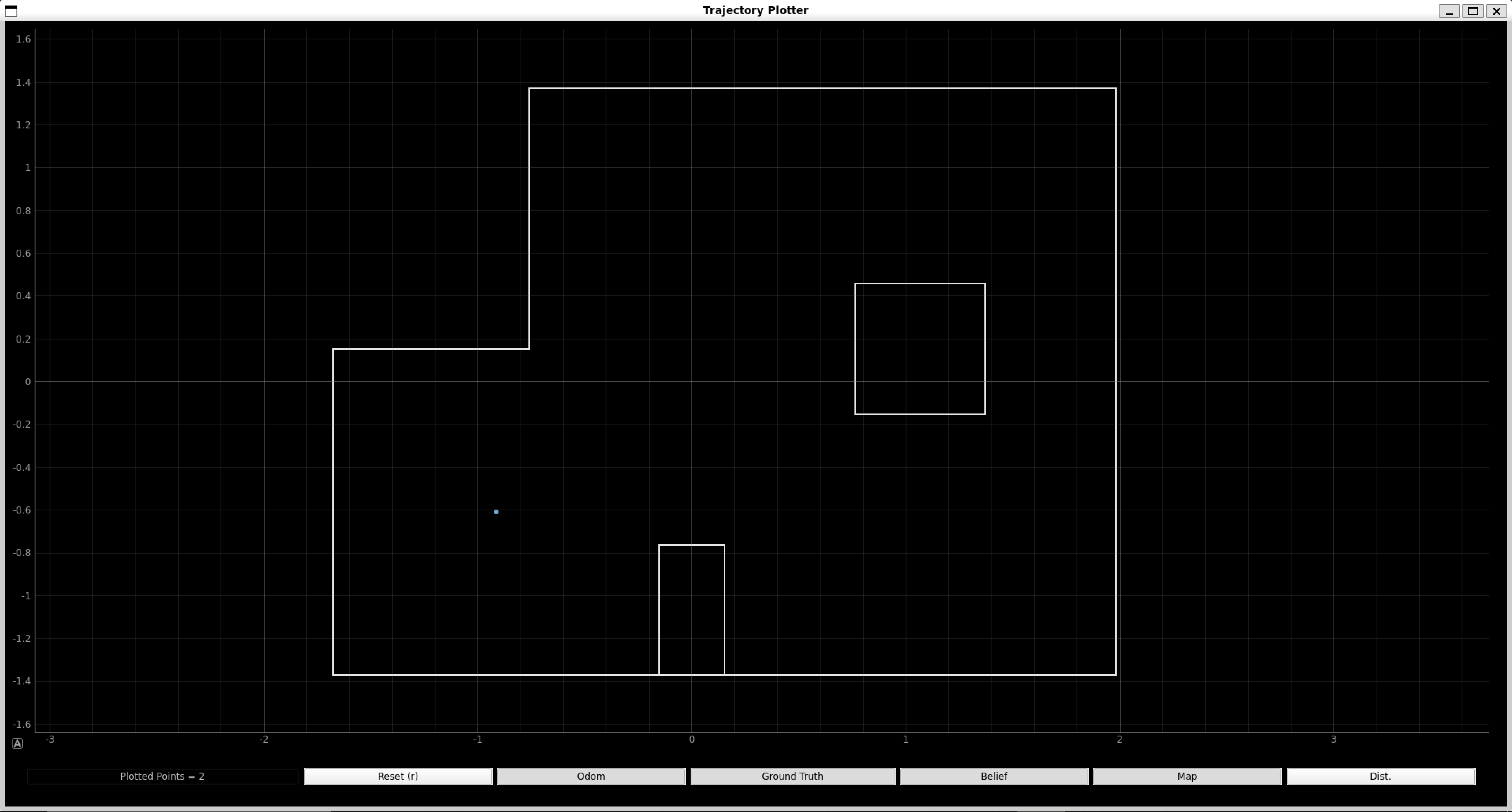

Our localization pose with respect to the ground truth was very close--either same (bottom two) or within one grid square off (top two). I think the discrepancy comes from the fact that the robot turns a little off axis, like in a circle. Other possible reasons might be that we place the robot not exactly on top of the ground truth locations, uncertainties in the ToF readings, and the map being slightly crooked.
I think the robot localizes better for the bottom two compared to the top two due to that fact that the bottom two map is less complicated and more forgiving than the top two. Becuase the unique features like boxes are further from where we are localizing, I think the bottom localizations came our better. However, I think the dominant discrepancy is from out robot turning a little off axis by a different amount every time and by luck, some localizations come out better than others.
The goal of this lab is to perform robot navigation through a set of waypoints in the map as quickly and accurately as possible.
I collaborated with TianTian Li and Raphael Fortuna on this Lab!
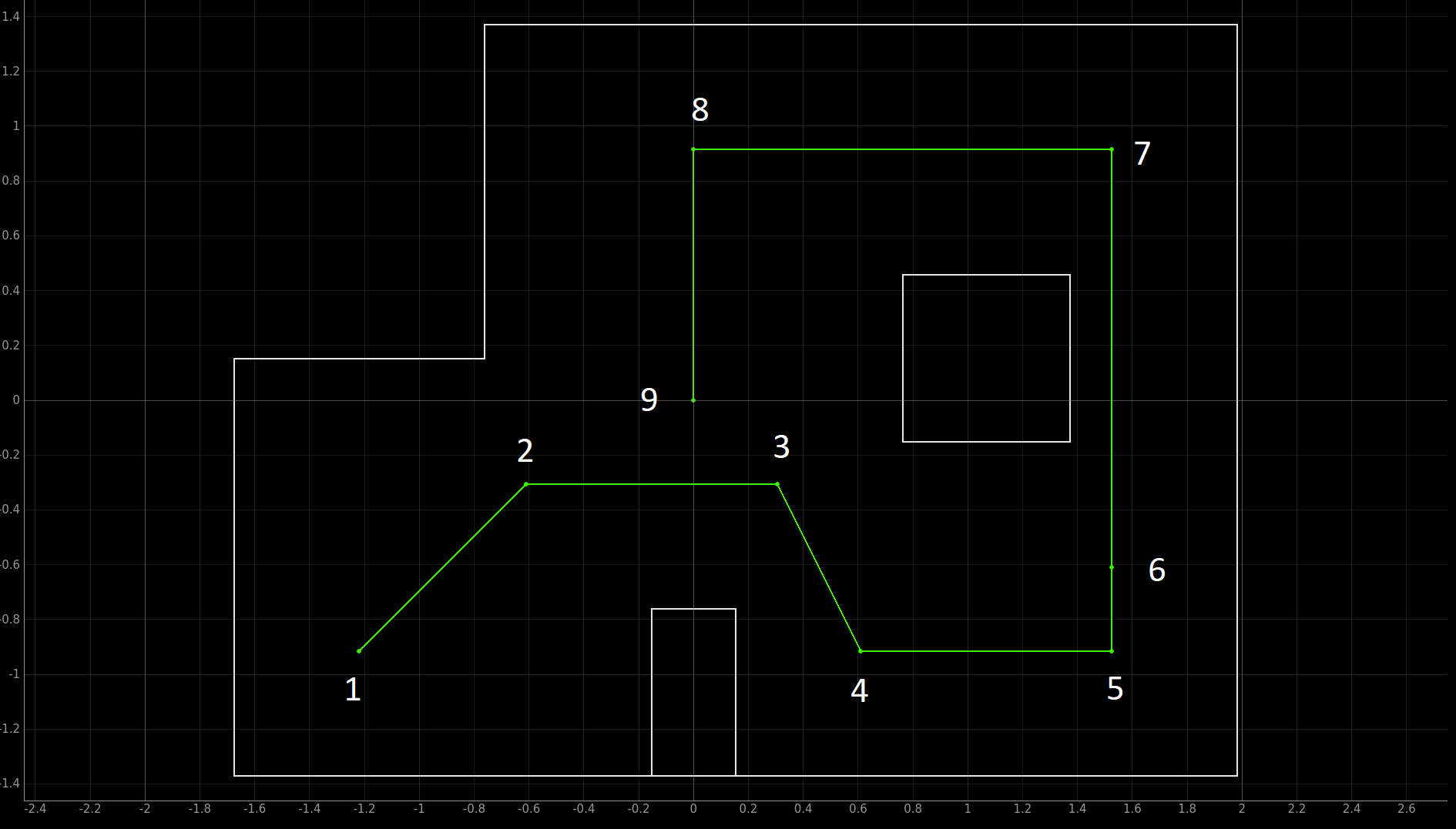
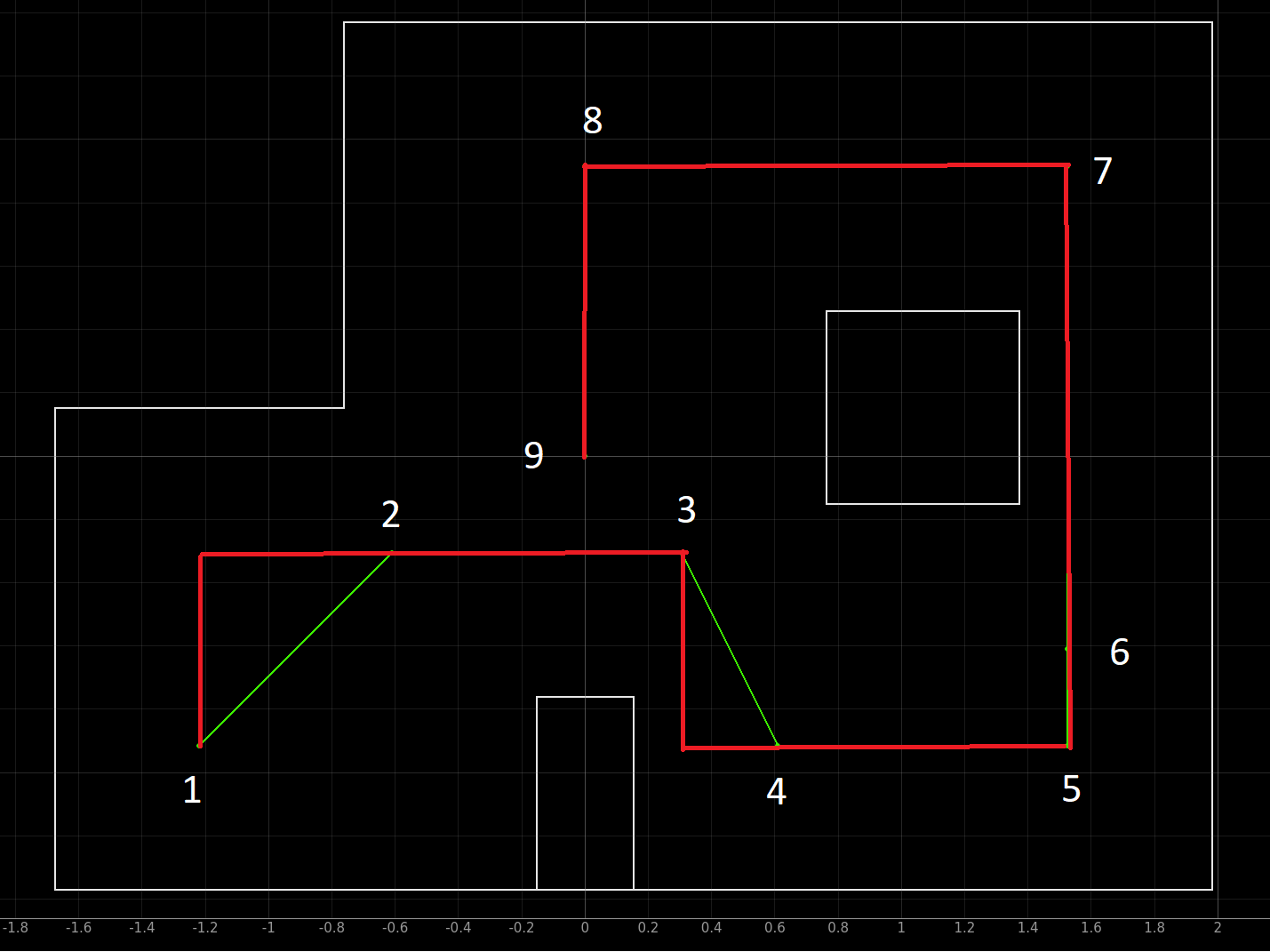
Waypoints that we have to hit are listed below:
1. (-4, -3) <--start
2. (-2, -1)
3. (1, -1)
4. (2, -3)
5. (5, -3)
6. (5, -2)
7. (5, 3)
8. (0, 3)
9. (0, 0) <--end
Since errors from the previous step propagte throughout the navigation, the later points get harder to hit. We tried out best to mitigate the error.
Our Attempts:
At first, we tried to use Bayes Filter and localize after getting to the each way point. However, we kept running into a problem where we get a different number of sample points even when we run the same code. In addition, depending on the battery level, our localization would end at a different angle, causing us trouble for the rest of the nagivation. In order to address this issue, we tried to use the magnetometer to tell us the ground truth angle so that we can correct for our heading angle. To do this, we made our robot stop so that the motor's magnetic field would not interfere with that of the magnetometer and took the measurement. Due to our sample number problem, we decided to use another method.
Our Plan:
We decided to go with closed loop gobal path planning method. Our computer would send commands for the robot to perform and the robot will not send back any data since we are not doing localization. When driving forward, we use Kalman Filter and PID. We use Kalman Filter to go a certain distance from where we are (e.g. we can tell it to go 1 ft). We use PID to go a certain distance from a wall (e.g. we can tell it to go 1 ft away from the wall). When turning, we use PID to get to get to a certain angle either through turning right or tunring left. We use this feedback system so that the robot can be move or turn more accurately. In terms of work distribution, I integrated the PID and Kalman Filter to move forward with the use of ToF, Tiantian integrated the PID turning for the IMU, and Raphael integrated the global path planning code for controlling the robot.
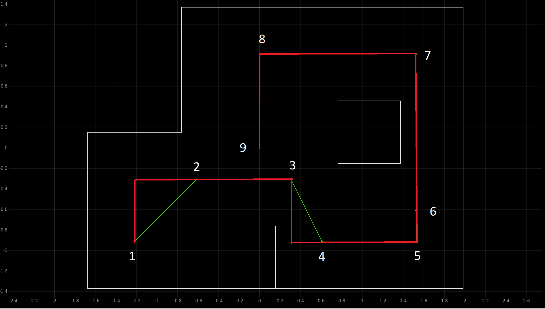
At first, we tried to take the shortest path to the waypoints. However, we found out that the ToF readings at an angle wasn't as accurate as we want it to be. So, we decided to create way points in the middle so that all of our robot rotations are all multiples of 90 degrees. Below is our new path shown in red.
Kalman Filter on Forward (distance from where it is at):
Below is our code snippet to do Kalman Filter to go a certain distance from it's location on ardunio. We already had a Kalman Filter implemented to go to a certain distance away from the wall in lab 7. So, we altered this code so that instead of going certain distance away from the wall, it goes a certain distance away from where it started. We accounted for the deadband in the motors by limiting the motor input to between 70 and 255. Kalman Filter along with ToF collecting 10 data points per second allowed us to react quickly to the changes. We used a Kp value of 0.4 determined in lab 7.
PID on Forward (distance away from wall):
Below is our code snippet to do proportional controller to get to a certain distance from the wall on arduino. We used PID to get to a distance away from the wall instead of doing Kalman Filter to get to a distance away from the wall because it was already implmented from lab 6 and worked great. Although the results will be barely any different, we could have implemented Kalman Filter to get to a certain distane away from the wall as we already have done so in lab 7. We accounted for the deadband in the motors by limiting the motor input to between 70 and 255. ToF collected 10 data points a second, which was quick enough for our use. We used a Kp value of 0.4, determined from lab 6.
PID on Turning:
Below is our code snippet to do proportional controller on turn right and turn left on arduino. We accounted for the deadband in the motors by limiting the motor input to between 100 and 200. The IMU collected 100 yaw data points per seconds. We used a Kp value of 1, determined in lab 6. We created seperate turn left and turn right commands to minimize the about of angle we turn to decrease gyroscope drift and error.
Path Planner:
The path planner was made to use the turn-go-turn procedure from the odometry model. We input our goal (x, y, yaw) points to the planner and the planner outputs that command to the robot. The command can be any of the four that we discussed above: PID on Forward, Kalman Filter on Forward, PID Turn Left, or PID Turn Right. We choose turn right or turn left depending on which turn takes less angle to achieve since gyroscope drift becomes more prominent as the angle increases. After each command is sent, the planner waits 5 or 10 seconds before sending the next command, depending on how long it takes to do that command.
As mentioned before, we added extra way points to avoid turning a non perpendicular turn. The path planer takes about 1.5 miliseonds to output the necessary commands to navigate through the entire map. The output was printed on Jupyter to be verified. Below is the code to do path planning.
Manual Adjustment:
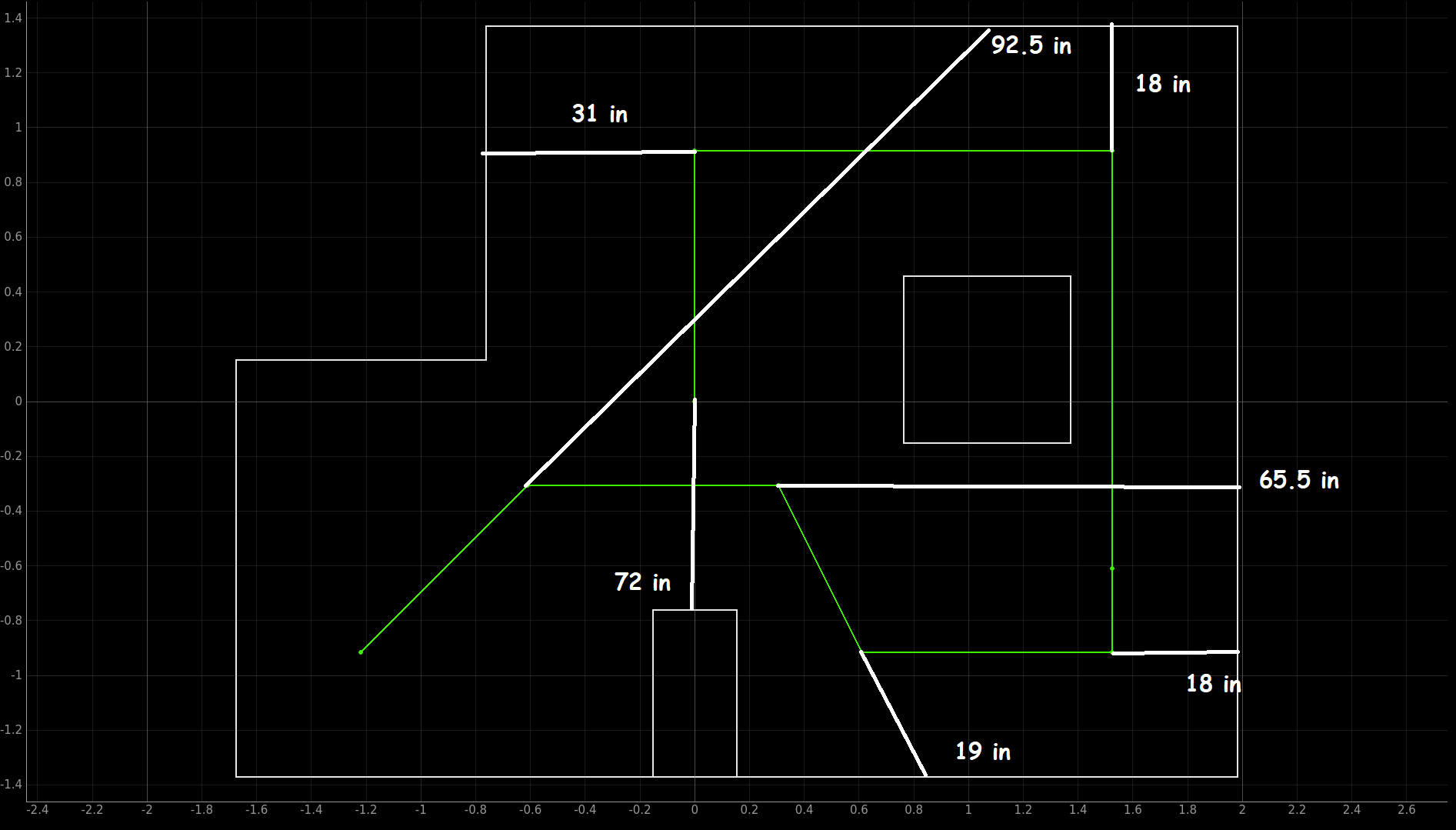
Based on our actual measurements of the map, as shown below, and from testing, we manually tuned our navigation code output from the path planner.
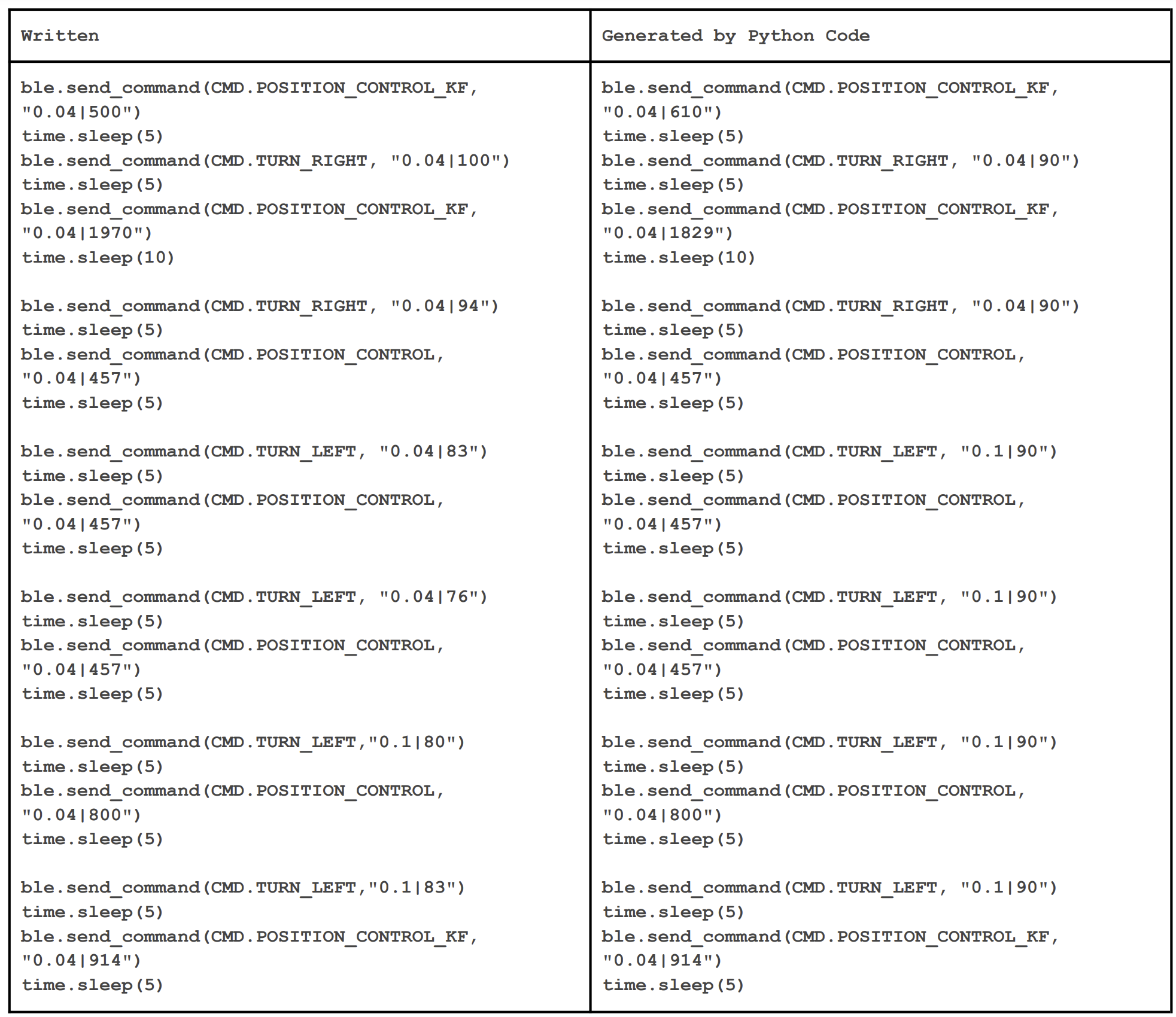
The right column below is our navigation code generated from the path planner. The left column below is our final code for nagivation that we ran.
As can be shown in the video, we were able to drive through or close to all the waypoints. As errors accumulated throughout the steps, it became harder to hit the later waypoints, espcially the last one. We tried our best, through steps outlined previously, to make our robot nagivate to all the way points accurately and quickly as possible. Thank you!
Our best run:
Our other runs: